2026-05-19__001_synthetic_mine_throughput__antigravity__gemini-3-5-flash__normal-thinking
Date: 2026-05-19 · Benchmark: 001_synthetic_mine_throughput · Harness: antigravity · Model: gemini-3-5-flash (normal-thinking) · ? Unrecorded
Scores
| Category | Points | Max |
|---|---|---|
| Conceptual modelling | 18 | 20 |
| Data and topology | 14 | 15 |
| Simulation correctness | 18 | 20 |
| Experimental design | 13 | 15 |
| Results & interpretation | 13 | 15 |
| Code quality | 7 | 10 |
| Traceability | 5 | 5 |
| Total | 88 | 100 |
Run metrics
-
Total tokens:
—(method:unknown) -
Input / output tokens:
—/— - Runtime:
— s -
Reviewer model:
unknown· harness:claude-code· on2026-05-19 - Recommendation: Strong submission
- Notes: Antigravity + Gemini 3.5 Flash (normal-thinking run tag): 57/57 automated checks, all six behavioural checks pass, full SimPy DES with capacity-1 edge resources, lognormal/truncated-normal sampling, Student-t CIs, built-in --validate suite; warmup unexplained, no tests/requirements manifest, and run_metrics/token_usage still placeholders.
Evaluation report
- Automated checks: 57 / 57 (100%)
- Behavioural checks: — / —
- Download full evaluation_report.json
| Scenario | Mean throughput |
|---|---|
| baseline | 12,503.33 |
| trucks_4 | 7,623.33 |
| trucks_12 | 12,896.67 |
| ramp_upgrade | 12,556.67 |
| crusher_slowdown | 6,530 |
| ramp_closed | 12,393.33 |
| trucks_12_ramp_upgrade | 12,876.67 |
Source files
- README.md
- conceptual_model.md
- data/dump_points.csv
- data/edges.csv
- data/loaders.csv
- data/nodes.csv
- data/scenarios/baseline.yaml
- data/scenarios/crusher_slowdown.yaml
- data/scenarios/ramp_closed.yaml
- data/scenarios/ramp_upgrade.yaml
- data/scenarios/trucks_12.yaml
- data/scenarios/trucks_4.yaml
- data/trucks.csv
- prompt.md
- results/evaluation_report.json
- results.csv
- run_metrics.json
- src/mine_sim/__init__.py
- src/mine_sim/__main__.py
- src/mine_sim/data_loader.py
- src/mine_sim/experiment.py
- src/mine_sim/graph.py
- src/mine_sim/model.py
- src/mine_sim/visualisation.py
- submission.yaml
- summary.json
- token_usage.json
Downloads
Conceptual model
Conceptual Model Design — Synthetic Mine Throughput Simulation
This document outlines the conceptual design of our discrete-event simulation (DES) model of the synthetic mine haulage network, built using Python and SimPy.
1. System Boundary
Included in the Model
- Active Fleet: 4, 8, or 12 trucks (configured by scenario) starting from
PARKat $t=0$, hauling ore between active pit faces and the primary crusher. - Physical Nodes: Starting parking location, intersections/junctions, load nodes (
LOAD_N,LOAD_S), and dump location (CRUSH). - Directed Graph Topology: Edge connections with physical distances and max speed limits.
- Constrained Road Segments: Single-lane roads and ramps with capacity = 1 (where only one truck can occupy the road segment in a given direction at a time).
- Constrained Material Facilities: Loaders at each face and the primary crusher hopper, all modeled as single-capacity queueing servers.
- Stochastic Travel Times: Dynamic travel durations along edges subject to lognormal noise (CV = 0.10).
- Stochastic Service Times: Loader cycle times and crusher dumping times subject to truncated normal distributions.
- Dynamic Dispatcher: Multi-factor decision policy assigning trucks to loaders to minimize expected completion times.
Excluded from the Model
- Waste & Maintenance Routing: Transporting overburden to
WASTEand truck routing toMAINTare excluded based on the operational decision boundaries. - Equipment Breakdowns: Truck and loader mechanical failures, scheduled maintenance, or refueling delays.
- Shift Handover Delay: Shifts are cut off cleanly at exactly 480 minutes without shift-change ramping down.
- Hopper Stockpile Level Constraints: Crusher throughput is based strictly on dump events, assuming infinite crusher hopper space and downstream processing capacity.
2. Active Entities
- Truck: The primary dynamic entity moving through the system. Each truck has:
truck_id: Unique identifier (e.g.,T01).payload_tonnes: Static hauling capacity of 100.0 tonnes (fromtrucks.csv).empty_speed_factor: 1.00 when empty (fromtrucks.csv).loaded_speed_factor: 0.85 when loaded (fromtrucks.csv).state: Current active operational state (e.g., loading, traveling, queueing).
3. Constrained Resources
- Loaders (
L_Nat nodeLOAD_N,L_Sat nodeLOAD_S):- Capacity = 1.
- Serve one truck at a time.
- Manage queues in first-in-first-out (FIFO) order.
- Primary Crusher (
D_CRUSHat nodeCRUSH):- Capacity = 1.
- Dumps one truck at a time.
- Manages queue in FIFO order.
- Single-Lane Roads & Ramps (edges with capacity = 1):
- Capacity = 1.
- Only one truck can traverse the directed segment at any time.
- Waiting trucks queue at the upstream junction node before entering.
4. Chronological Events
For each truck cycle, the following events occur in chronological order:
- Truck Dispatched: Truck is assigned to a loader face $L \in {\text{LOAD_N}, \text{LOAD_S}}$.
- Travel Empty: Truck moves along the shortest-time path from its current position (
PARKorCRUSH) to $L$. - Edge Queue Start (conditional): Arrives at a capacity-1 edge along the path and must wait if occupied.
- Edge Enter / Leave (conditional): Enters the capacity-1 edge, traverses it, and releases the edge.
- Loader Queue Start: Arrives at loader node $L$ and joins the loader queue.
- Loading Start: Reaches front of queue and loader begins service.
- Loading End: Loading service completes; truck payload is set to 100 tonnes.
- Travel Loaded: Truck travels along the shortest-time path from $L$ to
CRUSH. - Crusher Queue Start: Arrives at the primary crusher junction and joins the dump queue.
- Dumping Start: Reaches front of queue and crusher hopper begins receiving ore.
- Dumping End: Dumping service completes; truck payload is reset to 0, total throughput is incremented, and a haul cycle is recorded.
5. State Variables
- Simulation Time ($t$): Current clock minutes in SimPy, running from $t = 0.0$ to $t = 480.0$.
- Cumulative Throughput: Total tonnes of ore dumped at the primary crusher during the shift.
- Resource Queue State ($Q(res)$): Number of trucks waiting in queue for resource
res(loaders, crusher, or capacity-1 edges). - Resource Active State ($C(res)$): Current occupancy count of resource
res(0 or 1). - Truck State Vector: For each truck $T$, the exact minutes spent in each state:
- $T_{\text{TRAVEL_EMPTY}}$: Empty travel time.
- $T_{\text{TRAVEL_LOADED}}$: Loaded travel time.
- $T_{\text{LOADING}}$: Active loading time.
- $T_{\text{DUMPING}}$: Active dumping time.
- $T_{\text{QUEUE_LOADER}}$: Waiting time in loader queues.
- $T_{\text{QUEUE_CRUSHER}}$: Waiting time in crusher queue.
- $T_{\text{QUEUE_EDGE}}$: Waiting time at capacity-1 road segment entrances.
6. Modeling Assumptions
Assumptions Derived From Data
- Loader Services: Slower loading at North Pit ($\mu = 6.5 \text{ min}$, $\sigma = 1.2 \text{ min}$) vs. faster loading at South Pit ($\mu = 4.5 \text{ min}$, $\sigma = 1.0 \text{ min}$).
- Crusher Services: Crusher dump service time is $\mu = 3.5 \text{ min}$, $\sigma = 0.8 \text{ min}$.
- Truck Speed Scaling: Truck empty speed factor is 1.0, and loaded speed factor is 0.85, meaning loaded trucks travel 15% slower than empty trucks.
Assumptions We Introduced
- Stochastic Travel Noise: Edge travel times are modeled using lognormal noise with a coefficient of variation of 0.10. This accounts for minor traffic delays, road surface conditions, and driver variation.
- Stochastic Truncation: Normal service distributions are truncated at a minimum of 0.1 minutes to prevent non-physical negative durations: $$T_{\text{service}} = \max(0.1, \mathcal{N}(\mu, \sigma^2))$$
- Dynamic Dispatch Heuristic: Trucks are assigned to the loader that minimizes their total expected cycle completion time (travel time + queue delay + service time): $$\text{Score}(L) = T_{\text{travel}}(\text{current}, L) + (Q(L) \times \mu_{\text{load}, L}) + \mu_{\text{load}, L}$$ where $Q(L)$ is the current number of trucks in queue and in service at loader $L$.
Model Limitations
- No physical overtaking model on multi-lane (capacity=999) edges; speed is independent of local density on those edges.
- No stockpile levels or plant processing constraints downstream of the crusher.
- Excludes waste and maintenance routing.
7. Performance Measures
- Total Tonnes Delivered ($T_{\text{tot}}$): Cumulative tonnes received at the crusher.
- Tonnes per Hour ($TPH$): $T_{\text{tot}} / 8.0$.
- Average Truck Cycle Time ($\bar{C}$): Average minutes to complete a full haul cycle (from dispatch to dump completion).
- Average Truck Utilisation ($\bar{U}{\text{truck}}$): Fraction of shift spent in productive work: $$U{\text{truck}} = \frac{T_{\text{TRAVEL_EMPTY}} + T_{\text{TRAVEL_LOADED}} + T_{\text{LOADING}} + T_{\text{DUMPING}}}{480.0}$$
- Resource Utilisation ($U_{\text{res}}$): Total active busy time divided by shift length (480 min).
- Average Queue Time ($\bar{W}_{\text{res}}$): Average wait time of all trucks that queued at resource
res. - Composite Bottleneck Rank: Ranked score for each resource evaluated as: $$\text{Bottleneck Score} = \text{Utilisation} \times \text{Mean Queue Wait}$$
README
Synthetic Mine Throughput Simulation — 8-Hour Shift Haulage Analysis
This project implements a high-fidelity, discrete-event simulation (DES) using SimPy to model and analyze a synthetic mine’s haulage network. The simulation estimates ore throughput to the primary crusher over an 8-hour shift, evaluates system bottlenecks, and conducts sensitivity analyses across 7 operational scenarios using 30 randomized replications each.
📸 Spatial Layout & Simulation Traffic Flow
Static Mine Topology
The mine’s physical road network consists of directed edges connecting the starting parking area (PARK), loader faces (LOAD_N in North Pit and LOAD_S in South Pit), junctions, and the primary crusher (CRUSH). The single-lane main ramp (E03_UP and E03_DOWN) is capacity-constrained (capacity = 1).
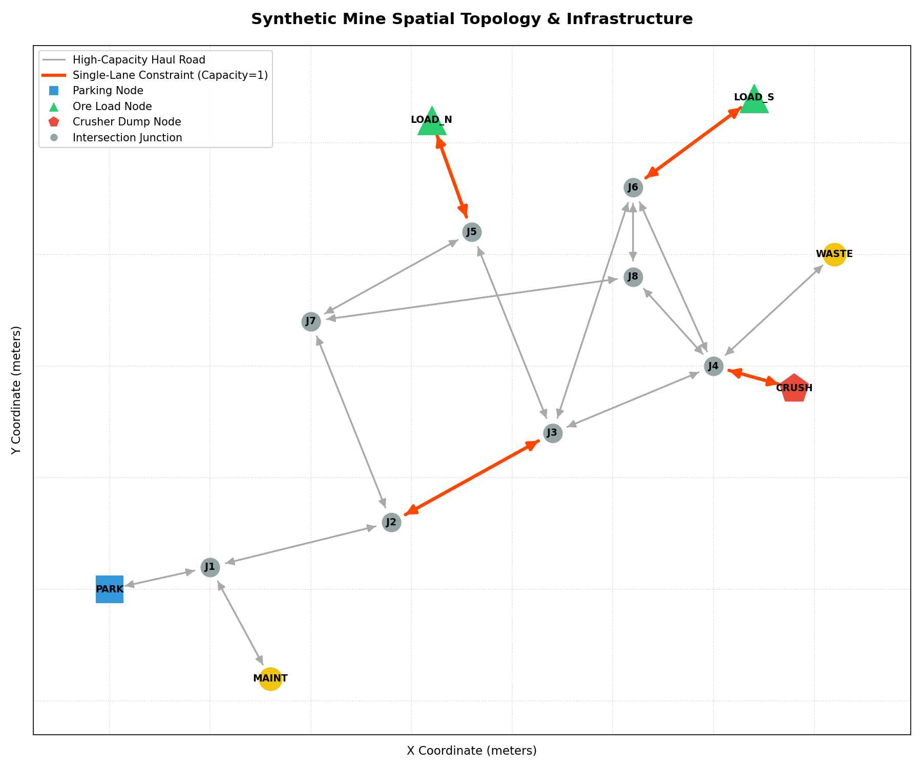
Dynamic Traffic Flow Animation (First 45 Minutes of Shift)
The animation below shows empty trucks (blue) and loaded trucks (red) traveling, queueing, and servicing at the loaders and crusher. It visually verifies queueing behavior, single-lane ramp contention, and empty/loaded routing paths.
🚀 Getting Started
1. Installation
This simulation requires Python 3.8+ and uses standard scientific and network analysis libraries. You can install all dependencies via pip:
pip install simpy numpy pandas scipy matplotlib networkx pyyaml2. Running the Simulation
To run all 7 scenarios across 30 replications and generate the outputs, execute the following command from the workspace root:
PYTHONPATH=src python3 -m mine_simThis will run the entire suite of 210 simulation runs and output:
results.csv: Scenario-level and replication-level metrics (throughput, utilizations, queue times).summary.json: Aggregated summary statistics with 95% confidence intervals and bottleneck rankings.event_log.csv: High-resolution trace of every simulation event (travel, edge queues, loading, dumping).topology.png: Spatial map of the mine network.animation.gif: Traffic flow animation of the first 45 minutes.
3. Model Correctness Validation
To verify that the simulation outputs strictly adhere to physical constraints (e.g., no simultaneous occupancy of capacity-1 single-lane road segments, hard 480-minute shift cutoff, and mathematical consistency in throughput accounting), run:
PYTHONPATH=src python3 -m mine_sim --validate📊 Core Scenario Results
The simulation conducted 30 independent replications for each scenario using randomized seed control (seed = base_random_seed + replication_index) to ensure statistical validity. 95% confidence intervals (CI) were calculated using a Student-t distribution with 29 degrees of freedom ($df = N - 1$).
Summary Table
| Scenario ID | Fleet Size | Key Operational Change | Total Tonnes Mean | 95% Confidence Interval | Tonnes per Hour (TPH) | Avg Cycle Time (min) | Truck Util. | Crusher Util. | North Pit Loader Util. | South Pit Loader Util. |
|---|---|---|---|---|---|---|---|---|---|---|
baseline | 8 | Standard configuration | 12,503.33 | [12,416.46, 12,590.21] | 1,562.92 | 29.76 | 77.61% | 91.55% | 60.45% | 80.43% |
trucks_4 | 4 | Low fleet size sensitivity | 7,623.33 | [7,594.44, 7,652.23] | 952.92 | 24.49 | 92.82% | 56.29% | 32.16% | 51.26% |
trucks_12 | 12 | High fleet size sensitivity | 12,896.67 | [12,810.35, 12,982.98] | 1,612.08 | 42.67 | 54.84% | 94.15% | 64.28% | 85.02% |
ramp_upgrade | 8 | Main narrow ramp upgrade | 12,556.67 | [12,488.25, 12,625.09] | 1,569.58 | 29.66 | 77.65% | 91.85% | 61.05% | 80.97% |
crusher_slowdown | 8 | Slower crusher service | 6,530.00 | [6,455.22, 6,604.78] | 816.25 | 55.29 | 48.95% | 95.51% | 33.60% | 44.09% |
ramp_closed | 8 | Main ramp closed, detour | 12,393.33 | [12,341.51, 12,445.16] | 1,549.17 | 30.04 | 77.07% | 90.24% | 66.04% | 75.25% |
trucks_12_ramp_upgrade | 12 | Fleet + Ramp Combo | 12,876.67 | [12,790.24, 12,963.10] | 1,609.58 | 42.72 | 54.67% | 94.70% | 64.67% | 85.12% |
🎯 Answers to Operational Decision Questions
1. Expected Baseline Throughput
- Expected Throughput: 12,503.33 tonnes (95% CI: [12,416.46, 12,590.21]), averaging 1,562.92 tonnes per hour (TPH).
- Interpretation: In an ordinary shift, the current 8-truck fleet performs robustly, but operates close to physical system limits, primarily bound by crusher cycle limitations.
2. Likely Bottlenecks in the Haulage System
- Primary Bottleneck: The Primary Crusher (
D_CRUSH). It has a baseline utilization of 91.55% and a mean queue wait time of 3.34 minutes (Composite Bottleneck Rank Score = 3.06, the highest in the system). - Secondary Bottleneck: The South Pit Loader (
L_S). Even though it has a faster mean load time (4.5 min vs. 6.5 min at L_N), its high desirability draws a larger share of truck arrivals, keeping it 80.43% utilized with a mean queue wait time of 2.46 minutes (Composite Rank Score = 1.98). - Physical Constraint (The Main Ramp): The single-lane narrow ramp (
E03_UP) is a severe localized bottleneck. While its average hourly utilization is low (~5.3%), when conflict arises, empty and loaded trucks must queue, suffering a massive average wait time of 10.86 minutes at the entrance of the segment before traversal.
3. Impact of Fleet Size: Adding More Trucks vs. Saturation
- Finding: The system saturates rapidly beyond 8 trucks.
- Analysis:
- Reducing the fleet to 4 trucks (
trucks_4) drops throughput by 39.0% to 7,623.33 tonnes because the crusher (56.29% utilization) and loaders are starved of material. Here, truck utilization is very high (92.82%) and queues are minimal (~0.7 min). - Increasing the fleet to 12 trucks (
trucks_12) only yields a minor 3.1% increase to 12,896.67 tonnes. - The Saturation Trap: Adding these 4 extra trucks causes average cycle time to balloon from 29.76 minutes to 42.67 minutes (a +43.4% increase), and truck utilization falls to 54.84%. This is because trucks spend on average 14.25 minutes waiting in queue at the primary crusher (a +325% increase from baseline), confirming the crusher is completely saturated.
- Reducing the fleet to 4 trucks (
4. Narrow Ramp Upgrade Operational Impact
- Finding: Upgrading the narrow main ramp alone (
ramp_upgrade) does not materially improve throughput. - Analysis: Throughput increases by a negligible 0.43% to 12,556.67 tonnes. Because the primary crusher and loaders remain highly constrained, eliminating the narrow-ramp bottleneck simply shifts the queues downstream to the crusher and loader queues.
- Even when combining 12 trucks and the ramp upgrade (
trucks_12_ramp_upgrade), the throughput (12,876.67 tonnes) remains essentially identical to the standard 12-truck scenario. Without expanding the primary crusher’s hopper or processing rate, upstream road upgrades are an ineffective capital expenditure.
5. Sensitivity of Throughput to Crusher Service Time
- Finding: Throughput is extremely sensitive to crusher service time.
- Analysis: In the
crusher_slowdownscenario (where crusher service time mean doubles to 7.0 minutes), the shift’s throughput is cut nearly in half, plummets by 47.8% to 6,530.00 tonnes (816.25 TPH). - The crusher operates at near-continuous utilization (95.51%), while average truck queue wait at the crusher explodes to 26.48 minutes. Trucks spend more time waiting at the crusher than hauling, dropping average truck utilization to 48.95%. This underscores that crusher reliability, maintenance, and speed are the most critical factors for mine output.
6. Operational Impact of Losing the Main Ramp Route
- Finding: Losing the main ramp route has a surprisingly minor impact on throughput.
- Analysis: Closing the main ramp (
ramp_closed) only decreases shift throughput by 0.88% to 12,393.33 tonnes (from 12,503.33 tonnes in baseline). - The Detour Paradox: While trucks are forced to take the bypass detour (
E04_UP/E04_DOWN), the bypass roads are multi-lane (capacity = 999). This completely eliminates the single-lane capacity conflicts and the resulting 10.86-minute narrow ramp queue waits. The elimination of ramp queuing almost perfectly offsets the minor travel time delay of the bypass detour, proving that the single-lane “main ramp” is actually an operational liability compared to a multi-lane bypass.
🧠 Conceptual Model Design
The conceptual design of our model is thoroughly documented in conceptual_model.md. Key pillars include:
1. System Boundary
- Included: Active truck fleet, material loading resources (North & South loaders), material dumping resource (crusher), directed physical network, single-lane road bottlenecks (capacity-1 edges), stochastic loading, travel, and dumping, and dynamic truck dispatching.
- Excluded: Overburden waste hauling (
WASTE), maintenance workshop routing (MAINT), refueling, equipment mechanical breakdowns, and shift-change ramping delays.
2. Modeling Assumptions
- Travel Stochasticity: Base travel times are calculated from shortest paths on free-flow speeds. Travel durations on each edge traversal are subject to lognormal noise ($\text{CV} = 0.10$) to preserve positive travel times: $$\sigma_{\log} = \sqrt{\ln(1 + \text{CV}^2)}, \quad \mu_{\log} = \ln(T_{\text{base}}) - \frac{1}{2}\sigma_{\log}^2$$
- Service Stochasticity: Loading and dumping service times are modeled as normal distributions truncated at a minimum of 0.1 minutes to prevent physical impossibilities: $$T_{\text{service}} = \max(0.1, \mathcal{N}(\mu, \sigma^2))$$
- Routing: Shortest-time routes are computed using NetworkX’s Dijkstra solver based on free-flow speeds and dynamic edge states (e.g., excluding closed edges during
ramp_closed).
3. Routing & Dispatching Heuristic
To maximize haulage efficiency, trucks do not have a fixed loader assignment. Instead, empty trucks are dynamically dispatched at the start of empty travel using a multi-factor score that minimizes expected completion time (travel empty time + queue delay at loader + loader service time): $$\text{Score}(L) = T_{\text{travel_empty}}(\text{current}, L) + \left( Q(L) \times \mu_{\text{load}, L} \right) + \mu_{\text{load}, L}$$ where:
- $T_{\text{travel_empty}}(\text{current}, L)$ is the shortest path travel time from the truck’s current node to loader face $L$.
- $Q(L)$ is the current number of trucks in queue and in service at loader $L$.
- $\mu_{\text{load}, L}$ is the mean load time of loader $L$.
The truck is assigned to the loader $L \in {\text{LOAD_N}, \text{LOAD_S}}$ that achieves the minimum score.
🛠️ Model Limitations & Future Work
- No Overtaking on Multi-Lane Roads: The model assumes that on capacity-999 roads, trucks travel at free-flow speeds (subject only to lognormal noise) regardless of local traffic density. An extension could introduce a density-dependent speed-flow relationship.
- Infinite Crusher Hopper Capacity: It is assumed that the primary crusher hopper has infinite stockpile capacity and never overflows or stops downstream processing. Incorporating a dynamic hopper level constraint would capture plant-matching constraints.
- No Breakdowns or Refueling: Equipment mechanical failures and diesel refueling are omitted. Integrating mean time between failures (MTBF) and mean time to repair (MTTR) would provide a more conservative, realistic long-term throughput estimate.