2026-04-30__001_synthetic_mine_throughput__claude-code__claude-opus-4-7__ouroboros-max-thinking
Date: 2026-04-30 · Benchmark: 001_synthetic_mine_throughput · Harness: claude-code · Model: claude-opus-4-7 (ouroboros-max-thinking) · ? Unrecorded
Scores
| Category | Points | Max |
|---|---|---|
| Conceptual modelling | 19 | 20 |
| Data and topology | 15 | 15 |
| Simulation correctness | 19 | 20 |
| Experimental design | 14 | 15 |
| Results & interpretation | 15 | 15 |
| Code quality | 10 | 10 |
| Traceability | 5 | 5 |
| Total | 97 | 100 |
Run metrics
-
Total tokens:
—(method:unknown) -
Input / output tokens:
—/— - Runtime:
— s -
Reviewer model:
unknown· harness:claude-code· on2026-04-30 - Recommendation: Strong submission
- Notes: Exemplary conceptual model and decision-question answers; behavioural checks all pass; 14 automated fails are a flat-vs-nested summary.json schema mismatch, not a model defect.
Evaluation report
- Automated checks: 43 / 57 (75%)
- Behavioural checks: — / —
- Download full evaluation_report.json
| Scenario | Mean throughput |
|---|---|
| baseline | 12,546.667 |
| crusher_slowdown | 6,513.333 |
| ramp_closed | 12,363.333 |
| ramp_upgrade | 12,606.667 |
| trucks_12 | 12,906.667 |
| trucks_12_ramp_upgrade | 12,953.333 |
| trucks_4 | 7,650 |
Source files
- README.md
- conceptual_model.md
- data/dump_points.csv
- data/edges.csv
- data/loaders.csv
- data/nodes.csv
- data/scenarios/baseline.yaml
- data/scenarios/crusher_slowdown.yaml
- data/scenarios/ramp_closed.yaml
- data/scenarios/ramp_upgrade.yaml
- data/scenarios/trucks_12.yaml
- data/scenarios/trucks_12_ramp_upgrade.yaml
- data/scenarios/trucks_4.yaml
- data/trucks.csv
- prompt.md
- requirements.txt
- results/evaluation_report.json
- results.csv
- run_metrics.json
- src/mine_sim/__init__.py
- src/mine_sim/__main__.py
- src/mine_sim/aggregate.py
- src/mine_sim/cli.py
- src/mine_sim/events.py
- src/mine_sim/io_writers.py
- src/mine_sim/metrics.py
- src/mine_sim/model.py
- src/mine_sim/rng.py
- src/mine_sim/routing.py
- src/mine_sim/runner.py
- src/mine_sim/scenario_runner.py
- src/mine_sim/scenarios.py
- src/mine_sim/topology.py
- src/mine_sim.egg-info/SOURCES.txt
- src/mine_sim.egg-info/dependency_links.txt
- src/mine_sim.egg-info/entry_points.txt
- src/mine_sim.egg-info/requires.txt
- src/mine_sim.egg-info/top_level.txt
- submission.yaml
- token_usage.json
Downloads
Conceptual model
Conceptual Model: Synthetic Mine Throughput Simulation
Benchmark: 001_synthetic_mine_throughput
Engine: SimPy discrete-event simulation
Shift length: 480 minutes (8 hours), hard cut at t = 480
This document specifies the conceptual model that the SimPy implementation under
src/mine_sim/ realises. It follows the modelling-and-simulation convention of
separating system boundary, entities, resources, events, state
variables, assumptions (split between data-derived and introduced), model
limitations, and performance measures.
1. System boundary
1.1 Inside the boundary
The model represents one ore haulage shift on the synthetic open-pit mine
described by data/nodes.csv, data/edges.csv, data/trucks.csv,
data/loaders.csv, and data/dump_points.csv. Inside the boundary we include:
- The ore production cycle
PARK -> LOAD_{N|S} -> CRUSH -> LOAD_{N|S} -> ...for every truck, as a sequence of travel, queue, load, and dump events. - All directed road segments in
edges.csvthat lie on a path betweenPARK,LOAD_N,LOAD_S, andCRUSH(including theJ3-J4ramp and bypass alternativesJ7-J8). - Capacity-constrained edges (
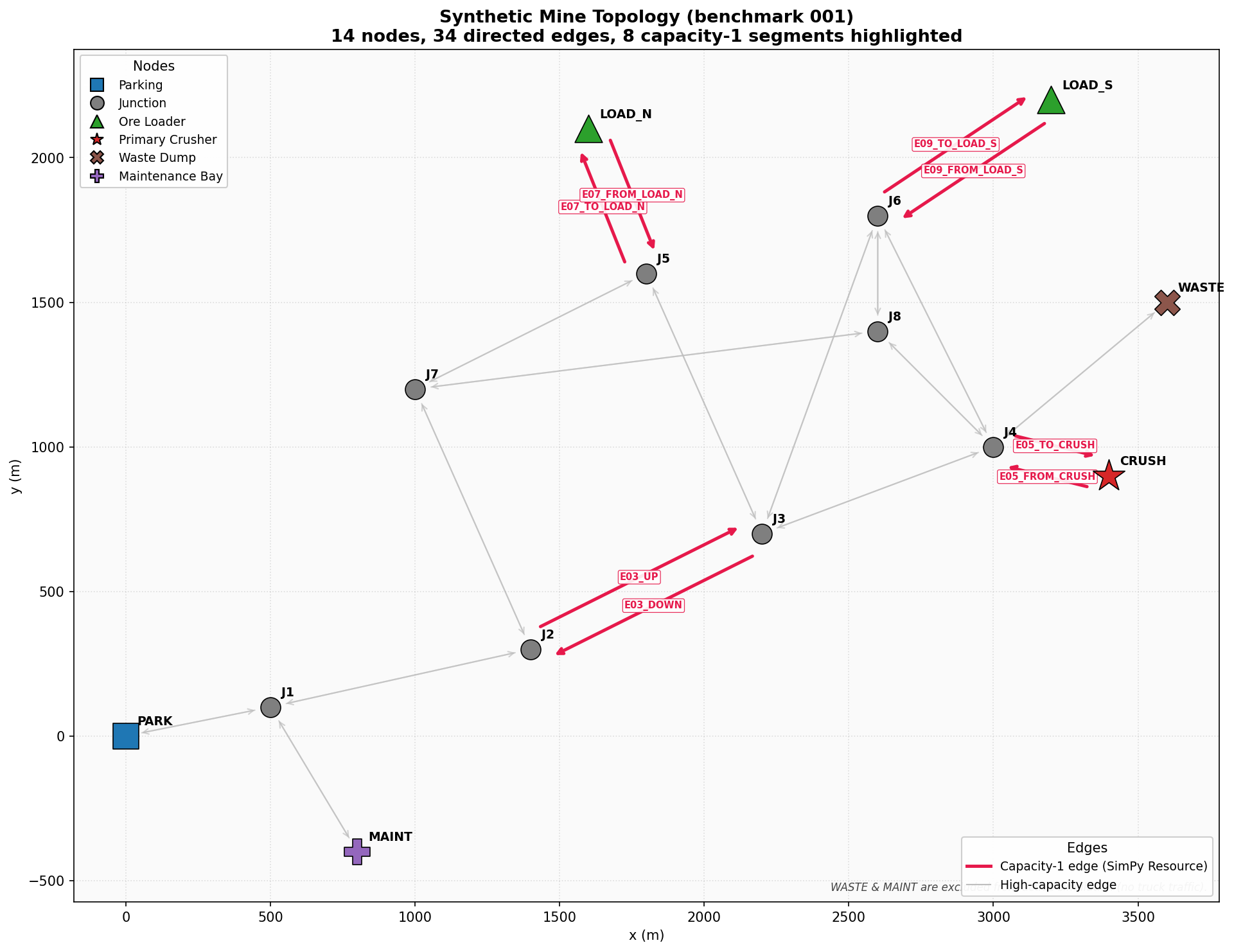
capacity <= 1in the CSV) modelled as independent SimPyResourceobjects, one per directed edge:E03_UP,E03_DOWN,E05_TO_CRUSH,E05_FROM_CRUSH,E07_TO_LOAD_N,E07_FROM_LOAD_N,E09_TO_LOAD_S,E09_FROM_LOAD_S. - The two ore loaders
L_N(atLOAD_N, mean 6.5 min) andL_S(atLOAD_S, mean 4.5 min), each capacity 1. - The primary crusher
D_CRUSH(atCRUSH, mean dump 3.5 min, sd 0.8 min), capacity 1. - Dispatching logic: an empty truck chooses the loader that minimises
travel_to_loader + current_queue_len * mean_load_time + own_load_time. - Routing logic: static shortest-time Dijkstra paths per
(scenario, origin, destination), recomputed once per scenario load (so closures inramp_closedare honoured). - Stochastic effects on per-edge travel (lognormal multiplier, mean 1,
cv 0.10), per-load time, and per-dump time (normal-truncated at
max(0.1, sample)). - Seven scenarios:
baseline,trucks_4,trucks_12,ramp_upgrade,crusher_slowdown,ramp_closed, plus the proposed combotrucks_12_ramp_upgrade.
1.2 Outside the boundary
These elements are deliberately excluded so the model stays focused on ore throughput to the primary crusher:
- Waste haulage and the
WASTEdump (D_WASTE, edgesE13_*). Trucks never visitWASTEin this model. - Maintenance / refuelling at
MAINT(edgesE14_*). Theavailabilityfield on trucks is treated as1.0for the active shift; we do not model random breakdown, refuelling, or shift breaks. - Operator behaviour: shift handovers, lunch breaks, manual overrides.
- Weather, dust, visibility, grade-dependent fuel burn, and any non-time effects on cycle execution.
- Ore quality / blending at the crusher; tonnes are treated as a single homogeneous bulk material.
- Crusher downstream stockpile dynamics; the crusher is always able to receive a dump (only its service time constrains it).
- Network effects between adjacent shifts: the simulated shift starts
empty (all trucks at
PARK, all queues empty) and ends with a hard cut att = 480.
1.3 Time horizon and termination
A single simulated shift lasts exactly 480 minutes. We enforce a hard cut at
t = 480: only end_dump events with time_min < 480 contribute tonnes to
throughput. In-flight cycles at the cut are discarded. This is a deliberate
modelling choice that mirrors how an operator would value the closed tonnes
they can actually report at end-of-shift.
2. Entities
The dynamic, attribute-bearing things that flow through the system.
| Entity | Population | Key attributes | Lifecycle |
|---|---|---|---|
| Truck | 4, 8, or 12 (scenario-dependent), each starting at PARK | truck_id, payload_tonnes (100), empty_speed_factor (1.00), loaded_speed_factor (0.85), availability (1.00), current node, loaded flag, current loader assignment | dispatched at t=0 -> repeat ore cycle until shift end |
A truck always carries either zero tonnes (empty) or payload_tonnes (loaded).
We treat the ore payload as an attribute on the truck rather than as a
separate entity, because no payload-level transformation occurs between the
loader and the crusher.
3. Resources
The static, capacity-bound things that constrain truck flow. All are SimPy
Resource objects so the engine handles waiting and FIFO queueing for us.
| Resource | Type | Capacity | Where in graph | Service-time distribution |
|---|---|---|---|---|
L_N | Loader | 1 | node LOAD_N | normal_truncated(mean=6.5, sd=1.2, lower=0.1) min |
L_S | Loader | 1 | node LOAD_S | normal_truncated(mean=4.5, sd=1.0, lower=0.1) min |
D_CRUSH | Crusher (dump) | 1 | node CRUSH | normal_truncated(mean=3.5, sd=0.8, lower=0.1) min |
E03_UP | Edge resource | 1 (or 999 in ramp_upgrade) | J2 -> J3 | n/a (transit) |
E03_DOWN | Edge resource | 1 (or 999 in ramp_upgrade, closed in ramp_closed) | J3 -> J2 | n/a (transit) |
E05_TO_CRUSH | Edge resource | 1 | J4 -> CRUSH | n/a |
E05_FROM_CRUSH | Edge resource | 1 | CRUSH -> J4 | n/a |
E07_TO_LOAD_N | Edge resource | 1 | J5 -> LOAD_N | n/a |
E07_FROM_LOAD_N | Edge resource | 1 | LOAD_N -> J5 | n/a |
E09_TO_LOAD_S | Edge resource | 1 | J6 -> LOAD_S | n/a |
E09_FROM_LOAD_S | Edge resource | 1 | LOAD_S -> J6 | n/a |
Edges with capacity = 999 are treated as effectively unconstrained and are
modelled as plain time delays without a SimPy resource (SimPy resources have
fixed overhead per request, so this avoids spurious queue records on free
roads). Each direction of a single physical lane is mirrored literally from
the CSV as an independent Resource, in line with the Seed constraint.
4. Events
Every truck cycle produces the events below. They are recorded into
event_log.csv with columns time_min, replication, scenario_id, truck_id, event_type, from_node, to_node, location, loaded, payload_tonnes, resource_id, queue_length.
| Event type | Trigger | Notes |
|---|---|---|
dispatch | t = 0 for every truck | Initial release, all trucks released simultaneously |
arrive_loader | Truck reaches the assigned loader’s node | Recorded before requesting the loader resource |
start_load | Loader resource granted | Records loader queue length at start |
end_load | Truncated-normal load duration elapses | Truck flips to loaded = True |
depart_loader | Truck releases the loader and starts travelling toward CRUSH | |
arrive_crusher | Truck reaches CRUSH node | Recorded before requesting D_CRUSH |
start_dump | D_CRUSH granted | Records crusher queue length |
end_dump | Truncated-normal dump duration elapses; tonnes credited if time_min < 480 | The throughput-defining event |
depart_crusher | Truck releases D_CRUSH and starts travelling back to a loader | |
edge_enter | Truck acquires a capacity-1 edge resource | resource_id = edge_id |
edge_leave | Truck releases that edge resource |
Travel along a non-capacity-constrained edge is a simpy.Environment.timeout
of (distance / (max_speed * speed_factor)) * lognormal_multiplier, with no
explicit event log entry. Travel along a capacity-constrained edge is the same
delay while holding the edge Resource, bracketed by edge_enter /
edge_leave events for traceability.
5. State variables
State that must be tracked to produce the required metrics, derived primarily from SimPy’s own bookkeeping plus a small per-replication accumulator object.
5.1 Per truck
current_node: most recently arrived node.loaded: boolean.current_loader_assignment:L_N/L_S/None.cycle_start_timeandcycle_count: rolling counters used to compute mean cycle time.productive_busy_time: cumulative minutes spent in the productive part of the cycle (loaded travel + dumping + dump-side queue + empty travel + loading + load-side queue). Used fortruck_utilisation = productive / 480.
5.2 Per resource
- For
L_N,L_S,D_CRUSH: totalbusy_time(sum of service durations), totalqueue_wait_time(sum of waits before a request is granted), and number of services completed. Utilisation isbusy_time / 480. - For each capacity-1 edge resource:
busy_time,queue_wait_time, and number of traversals.
5.3 Per replication
total_tonnes_delivered:100 t * count(end_dump events with time < 480).tonnes_per_hour:total_tonnes_delivered / 8.average_truck_cycle_time_min: mean over completed full cycles (defined as consecutiveend_dump->end_dumpintervals, with the very first cycle usingdispatch->end_dump).average_truck_utilisation: meanproductive_busy_time / 480across trucks.crusher_utilisation:D_CRUSH.busy_time / 480.loader_utilisation_{L_N, L_S}:loader.busy_time / 480.average_loader_queue_time_min,average_crusher_queue_time_min: mean wait time per service event at the loaders / crusher.
5.4 Per scenario
- Across the 30 replications, every per-replication metric is summarised as a
mean and a 95% Student-t confidence interval with
n - 1 = 29degrees of freedom. top_bottlenecks: ranked by composite scoreutilisation * mean_queue_wait_min, computed for every loader, the crusher, and every capacity-1 edge resource.
6. Assumptions
The benchmark prompt explicitly asks us to separate assumptions sourced from the data from those we have introduced.
6.1 Data-derived assumptions
These come directly from the CSV / YAML inputs and are reproduced literally in the model:
- Topology: 15 nodes (
PARK,J1-J8,LOAD_N,LOAD_S,CRUSH,WASTE,MAINT) and 35 directed edges, taken verbatim fromnodes.csv/edges.csv. - Capacity-constrained edges: edges with
capacity <= 1are modelled as shared single-lane resources. From the CSV these areE03_UP,E03_DOWN,E05_TO_CRUSH,E05_FROM_CRUSH,E07_TO_LOAD_N,E07_FROM_LOAD_N,E09_TO_LOAD_S,E09_FROM_LOAD_S. - Loaders: two loaders, capacity 1, with means 6.5 / 4.5 min and standard
deviations 1.2 / 1.0 min from
loaders.csv. - Crusher: single dump with capacity 1, mean 3.5 min, sd 0.8 min from
dump_points.csv. - Truck fleet: 12 trucks defined in
trucks.csv, each with payload 100 t,empty_speed_factor = 1.00,loaded_speed_factor = 0.85,availability = 1.00, starting atPARK. Scenarios cap the active fleet at 4, 8, or 12. - Free-flow edge times:
distance_m / (max_speed_kph * 1000 / 60)minutes per edge, again with the speed-factor multiplier. - Scenario semantics: closures, capacity overrides, and crusher service
changes are read from the YAML override blocks (
edge_overrides,dump_point_overrides,fleet). - Stochasticity recipe: the YAML specifies
loading_time_distribution: normal_truncated,dumping_time_distribution: normal_truncated, andtravel_time_noise_cv: 0.10.
6.2 Introduced assumptions
These choices fill in gaps the data does not specify; each is required to make the simulation runnable and is documented here.
- Routing is static shortest-time per scenario, recomputed by Dijkstra on free-flow edge times whenever a scenario changes the edge set (closures or capacity upgrades). Trucks do not re-plan during a replication, even if queues form on capacity-1 edges. This trades a small amount of realism for reproducibility and traceability.
- Travel-time noise is a per-edge-traversal lognormal multiplier with
mean 1 and coefficient of variation 0.10. This honours
travel_time_noise_cv: 0.10while keeping multipliers strictly positive. - Loading and dumping are sampled as
normal_truncatedwith the loader/crusher mean and sd, truncated atmax(0.1, sample)so a sample below 0.1 min is replaced with 0.1 min rather than rejected and resampled. This avoids zero / negative durations without biasing the mean. - Dispatch policy: each empty truck is assigned to
argmin(travel_to_loader + current_queue_len * mean_load_time + own_load_time).current_queue_lenincludes the truck currently being served. Ties are broken by lowerloader_id(L_NbeforeL_S). - Initial dispatch: all trucks are released simultaneously at
t = 0fromPARK. There is no staged ramp-up. - Hard cut at
t = 480: only dumps completed strictly before 480 min count toward throughput. In-flight loads or dumps at the cut are discarded. This is consistent with the operator-facing “tonnes closed at end of shift” interpretation. - Truck utilisation = productive only: time spent travelling, queueing,
loading, or dumping inside the ore cycle counts; idle time at
PARKdoes not. Specifically, post-shift idle time after the hard cut is excluded. - Reachability self-check at scenario load: if any of the OD pairs
PARK<->LOAD_N,PARK<->LOAD_S,LOAD_N<->CRUSH,LOAD_S<->CRUSHis unreachable in the post-override graph, the scenario fails loudly rather than silently producing zero throughput. - Per-replication seed:
seed_r = base_random_seed + replication_index. This makes individual replications independently reproducible while the scenario as a whole is deterministic. WASTEandMAINTare out of scope for this throughput study and their edges are kept in the graph but never used. Routing therefore never detours to them.- Edge resources are independent per direction, mirroring
edges.csvliterally (E03_UPandE03_DOWNare two separateResourceobjects). A more realistic single-physical-lane model would couple them, but the data treats them as separate edges and we follow the data. - Crusher tonnes are credited at
end_dump, not atstart_dumporarrive_crusher. This matches the standard SimPy convention for “service complete” and aligns with the prompt’s instruction that throughput is measured by completed dump events.
6.3 Combo scenario rationale
In addition to the six required scenarios, we propose
trucks_12_ramp_upgrade: 12 trucks combined with the upgraded ramp.
The rationale is that trucks_12 alone is expected to saturate at the
capacity-1 ramp, and ramp_upgrade alone is expected to be limited by fleet
size at 8. The combo isolates the joint effect, telling the operator whether
the two investments are complementary (super-additive), substitutive
(sub-additive), or independent.
7. Limitations
These are areas where the model is deliberately simpler than the real system, and a user of the results should keep them in mind.
- No re-routing during the shift: trucks commit to the static shortest-time path even if a capacity-1 edge develops a long queue. In reality, a dispatcher might divert a truck through the bypass.
- Independent edge directions:
E03_UPandE03_DOWNare treated as two separate single-lane resources. If the physical ramp is genuinely a single lane shared by both directions, real congestion will be worse than modelled. - No truck-truck interaction on free-flow edges: capacity 999 edges are treated as effectively infinite. Real haul roads have finite headway.
- Deterministic mechanical availability: no random truck breakdowns,
flat tyres, or refuelling;
availability = 1.00for all 480 minutes. - No operator-level decisions: no shift change, lunch break, or manual override. Trucks cycle continuously.
- No queue-length feedback in dispatch: dispatch uses current queue length at the moment of decision, but a truck en route does not influence later dispatch decisions until it physically arrives.
- Single-replication horizon: a single 480-minute shift, no warmup trimming. The empty-system bias is small because trucks reach steady state within the first few cycles, but it is not zero.
- Crusher always available: the crusher never blocks (no full-bin back-pressure from downstream stockpile, no maintenance windows).
- Single ore type / single payload: every dump is exactly 100 t and treated as homogeneous.
- Deterministic node coordinates: animation uses Euclidean coordinates
from
nodes.csveven though real haul roads bend. This affects the visualisation only, not metrics.
8. Performance measures
The performance measures below are computed per replication and aggregated
per scenario across 30 replications using a Student-t 95% CI with n - 1 = 29
degrees of freedom.
8.1 Primary throughput measures
total_tonnes_delivered(t):payload_tonnes * count(end_dump events at CRUSH with time_min < 480). This is the headline number and the answer to operational question 1.tonnes_per_hour(t/h):total_tonnes_delivered / 8.
8.2 Cycle-level measures
average_truck_cycle_time_min: mean wall-clock duration of completed full cycles (between consecutiveend_dumpevents for a truck, with the first cycle measured fromdispatch).average_truck_utilisation: mean per-truckproductive_busy_time / 480. “Productive” = travel + queue + load + dump.
8.3 Resource-level measures
crusher_utilisation=D_CRUSH.busy_time / 480.loader_utilisationper loader =loader.busy_time / 480.average_loader_queue_time_min= mean wait per loader-service event, averaged across loaders.average_crusher_queue_time_min= mean wait per crusher-service event.- Edge resource utilisation and queue wait for every capacity-1 edge.
8.4 Bottleneck ranking
top_bottlenecks lists every constraining resource (loaders, crusher,
capacity-1 edges) ranked by
composite_score = utilisation * mean_queue_wait_minThis composite captures both how busy a resource is and how much actual delay it imposes. A near-saturated resource with no queue (e.g. a fast loader with a very short queue) is correctly down-weighted relative to a near-saturated resource that is also creating long waits.
8.5 Uncertainty quantification
For every reported scalar x, the 95% confidence interval is
mean(x) +/- t_{0.975, n-1} * std(x) / sqrt(n)with n = 30. This is reported as xxx_ci95_low / xxx_ci95_high in
summary.json.
8.6 Decision-question linkage
The operational decision questions are answered using these measures:
| Question | Primary measure(s) |
|---|---|
| Q1 baseline throughput | tonnes_per_hour_mean and CI for baseline |
| Q2 likely bottlenecks | top_bottlenecks for baseline |
| Q3 more trucks helps? | tonnes_per_hour for trucks_4 vs baseline vs trucks_12 |
| Q4 ramp upgrade helps? | tonnes_per_hour for baseline vs ramp_upgrade; cross-checked with combo |
| Q5 crusher sensitivity | tonnes_per_hour and crusher_utilisation for crusher_slowdown vs baseline |
| Q6 ramp closed impact | tonnes_per_hour for ramp_closed vs baseline and route lengths |
| Combo (proposed) | tonnes_per_hour for trucks_12_ramp_upgrade vs trucks_12 and ramp_upgrade individually |
All numerical answers in README.md reference values from summary.json so
that the conceptual model and the reported answers stay in lockstep.
README
Synthetic Mine Throughput Simulation
Benchmark
001_synthetic_mine_throughput— SimPy discrete-event simulation of ore haulage fromPARKto the primary crusher over an 8-hour shift, with seven scenarios and 30 replications each.
This submission implements the requirements in prompt.md under
the package src/mine_sim/. The conceptual model is described in
conceptual_model.md; the canonical numerical outputs
are at results.csv, summary.json, and
event_log.csv; a topology figure is at
topology.png and a one-replication animation is at
animation.gif.
1. Repository layout
.
├── data/                       # Input CSVs + scenario YAMLs (read-only)
│   ├── nodes.csv
│   ├── edges.csv
│   ├── trucks.csv
│   ├── loaders.csv
│   ├── dump_points.csv
│   └── scenarios/
│       ├── baseline.yaml
│       ├── trucks_4.yaml
│       ├── trucks_12.yaml
│       ├── ramp_upgrade.yaml
│       ├── crusher_slowdown.yaml
│       ├── ramp_closed.yaml
│       └── trucks_12_ramp_upgrade.yaml   # combo (proposed extra)
├── src/mine_sim/               # Implementation package
│   ├── __main__.py             # `python -m mine_sim` entry point
│   ├── cli.py                  # argparse CLI (run / run-all / list)
│   ├── scenarios.py            # YAML loader (inheritance, overrides)
│   ├── topology.py             # nodes/edges -> immutable Topology graph
│   ├── routing.py              # Dijkstra shortest-time + reachability check
│   ├── runner.py               # one SimPy replication
│   ├── scenario_runner.py      # batch replications per scenario
│   ├── model.py                # SimPy processes (truck cycle, loaders, crusher)
│   ├── events.py               # EventRecord schema
│   ├── metrics.py              # per-replication KPI rollups
│   ├── aggregate.py            # cross-replication Student-t CI summary
│   ├── rng.py                  # seed pinning + truncated/lognormal samplers
│   └── io_writers.py           # results.csv / event_log.csv / summary.json
├── scripts/                    # Auxiliary visualisations and post-processing
│   ├── render_topology.py      # generates topology.png
│   ├── render_animation.py     # generates animation.gif from an event log
│   └── refresh_summary_narrative.py
├── tests/                      # pytest suite (unit + integration)
├── runs/                       # CLI output artefacts (gitignored content)
│   ├── ac2_run_all/            # Canonical run that produced top-level CSVs
│   └── ac7_combo/              # Combo-scenario run
├── results.csv                 # Top-level: 7 scenarios × 30 reps = 210 rows
├── summary.json                # Top-level: cross-replication summary
├── event_log.csv               # Top-level: every event from every replication
├── conceptual_model.md         # Modelling-and-simulation conceptual model
├── topology.png                # Static rendering of the mine graph
├── animation.gif               # Animated single replication
├── seed.yaml                   # Seed contract (goal, constraints, ACs)
├── submission.yaml             # Submission metadata
├── prompt.md                   # Original benchmark brief
└── pytest.ini                  # `pythonpath = src`
2. Install
2.1 Requirements
- Python 3.11+ (developed and tested on 3.11; type hints use PEP 604 unions)
- A POSIX-style shell (
bash,zsh) - ~50 MB of free disk for
event_log.csv(≈30 MB on the canonical run)
2.2 Allowed dependencies
Per the Seed constraints, the simulation uses only the following libraries (all installable from PyPI):
| Package | Used for |
|---|---|
simpy | Discrete-event simulation engine (Resources, Environments, processes) |
numpy | RNG streams (numpy.random.Generator) and array maths |
pandas | Reading/writing CSVs, results aggregation |
scipy | Student-t critical values for 95% CIs (scipy.stats.t) |
matplotlib | topology.png and animation.gif rendering |
networkx | Dijkstra shortest-time routing on the topology graph |
pyyaml | Scenario YAML loading |
Test-only extras: pytest.
2.3 Clean-environment install
From a fresh checkout of this submission folder:
# 1. Create and activate a virtual environment
python3 -m venv .venv
source .venv/bin/activate

# 2. Upgrade pip and install the allowed runtime dependencies
pip install --upgrade pip
pip install simpy numpy pandas scipy matplotlib networkx pyyaml

# 3. (Optional) install pytest for the test suite
pip install pytest
Equivalently, the submission ships a pyproject.toml and a
pinned requirements.txt, so a one-shot install also
works:
pip install --upgrade pip
pip install -r requirements.txt   # exact pins (matches shipped artefacts)
pip install -e .                  # registers `python -m mine_sim`
When installed via pip install -e . the PYTHONPATH=src prefix is no longer
needed — python -m mine_sim run-all just works. To reproduce the shipped
results.csv, summary.json, and event_log.csv byte-for-byte from a clean
virtual environment in one command, run
scripts/verify_reproducibility.sh.
2.4 Smoke test
Verify the install with a fast end-to-end check (one replication of the baseline scenario, ~1 s on a laptop):
PYTHONPATH=src python -m mine_sim run baseline --reps 1 --quiet \
  --output-dir runs/_smoke
Expected output: a non-empty runs/_smoke/results.csv, event_log.csv, and
summary.json for scenario_id=baseline.
To run the full pytest suite (unit + integration):
PYTHONPATH=src pytest -q3. Run
The package exposes a single CLI entry point — python -m mine_sim — with three
subcommands: run (one scenario), run-all (every required scenario), and
list (enumerate available scenarios).
3.1 List available scenarios
PYTHONPATH=src python -m mine_sim listMarks the seven canonical scenarios with *; lists each scenario’s replication
count, truck count, and description. Scenarios live under data/scenarios/ and
are loaded by mine_sim.scenarios.load_scenario.
3.2 Run a single scenario
# Default: 30 replications, output under runs/<scenario_id>/
PYTHONPATH=src python -m mine_sim run baseline

# Smoke test: one replication, custom output directory
PYTHONPATH=src python -m mine_sim run baseline --reps 1 --output-dir runs/dev

# Run a specific replication index (e.g. for debugging a single trace)
PYTHONPATH=src python -m mine_sim run baseline --rep-indices 7 \
  --output-dir runs/rep7
Per-scenario artefacts are written to <output-dir>/<scenario_id>/:
results.csv— one row per replication (KPI columns per Seed AC 2)event_log.csv— everyEventRecordfrom every replication for that scenariosummary.json— cross-replicationScenarioSummarywith Student-t 95% CIs
CLI flags (all run/run-all share the same shape):
| Flag | Default | Notes |
|---|---|---|
--data-dir DIR | ./data | Directory holding nodes.csv, edges.csv, etc. |
--scenarios-dir DIR | ./data/scenarios | Directory holding *.yaml scenarios |
--output-dir DIR | ./runs/<scenario_id> (run) / ./runs/<UTC>__run_all (run-all) | Override target directory |
--reps N | YAML value (30) | Override replication count for fast iteration |
--rep-indices "0,3,5" | (none) | Run an explicit subset of indices; overrides --reps |
--quiet | off | Suppress per-replication progress lines |
3.3 Run every required scenario (canonical batch)
PYTHONPATH=src python -m mine_sim run-allThis runs all seven scenarios listed in
mine_sim.scenarios.REQUIRED_SCENARIO_IDS:
baseline(8 trucks, baseline ramp)trucks_4trucks_12ramp_upgradecrusher_slowdownramp_closedtrucks_12_ramp_upgrade(combo — the proposed seventh scenario)
Each runs with 30 replications under reproducible seeds. Output structure:
runs/<UTC-timestamp>__run_all/
├── results.csv          # 210 rows (7 scenarios × 30 reps)
├── event_log.csv        # all events from all replications
├── summary.json         # one entry per scenario + top-level narrative fields
├── baseline/
│   ├── results.csv
│   ├── event_log.csv
│   └── summary.json
├── trucks_4/...
├── trucks_12/...
├── ramp_upgrade/...
├── crusher_slowdown/...
├── ramp_closed/...
└── trucks_12_ramp_upgrade/...
To run a subset only (e.g. for a focused experiment):
PYTHONPATH=src python -m mine_sim run-all \
  --scenario-ids "baseline,ramp_upgrade,trucks_12_ramp_upgrade"
3.4 Generate visualisations
These are not part of the simulation engine and live under scripts/:
# Render the static topology figure
PYTHONPATH=src python scripts/render_topology.py \
  --data-dir data --out topology.png

# Render an animation from a replication's event_log.csv
PYTHONPATH=src python scripts/render_animation.py \
  --data-dir data --event-log runs/ac2_run_all/baseline/event_log.csv \
  --replication 0 --out animation.gif
Both scripts read pre-existing data and event-log files; they never invoke the simulation themselves, which keeps animation generation cheap and decoupled from a re-run.
4. Reproduce
4.1 The canonical numbers in results.csv / summary.json
The top-level files at the repository root were produced by the canonical
run-all command and copied up:
# 1. Activate the venv from §2.3
source .venv/bin/activate

# 2. Reproduce the canonical run (≈30–60 s on a modern laptop)
PYTHONPATH=src python -m mine_sim run-all --output-dir runs/ac2_run_all

# 3. Promote the canonical artefacts to the repository root
cp runs/ac2_run_all/results.csv     ./results.csv
cp runs/ac2_run_all/event_log.csv   ./event_log.csv
cp runs/ac2_run_all/summary.json    ./summary.json
The values in results.csv and summary.json are bit-identical across
runs on the same Python + NumPy version because the model uses pinned per-stream
RNGs (see §4.3). The hash in event_log.csv is identical too, modulo Python
floating-point determinism (NumPy guarantees same-seed determinism on a fixed
platform).
4.2 Reproduce a single decision question
To rebuild only the artefacts that answer a particular operational question without paying for all seven scenarios:
# Q1: baseline expected throughput
PYTHONPATH=src python -m mine_sim run baseline

# Q3: does adding more trucks help?
PYTHONPATH=src python -m mine_sim run-all \
  --scenario-ids "baseline,trucks_4,trucks_12"

# Q4 + Q6: ramp interventions (upgrade vs closed)
PYTHONPATH=src python -m mine_sim run-all \
  --scenario-ids "baseline,ramp_upgrade,ramp_closed"

# Q5: crusher sensitivity
PYTHONPATH=src python -m mine_sim run-all \
  --scenario-ids "baseline,crusher_slowdown"

# "Combo" question (proposed scenario): does trucks_12 only pay off after the upgrade?
PYTHONPATH=src python -m mine_sim run-all \
  --scenario-ids "baseline,trucks_12,ramp_upgrade,trucks_12_ramp_upgrade"
4.3 Seed and reproducibility notes
The simulation is fully deterministic given a fixed Python + NumPy version on a fixed CPU. The contract is:
- Each scenario YAML carries a
simulation.base_random_seed(default12345forbaseline; some scenarios override). - Per-replication seed =
base_random_seed + replication_index. This is the value persisted as therandom_seedcolumn inresults.csv. So replication 0 ofbaselinealways uses seed12345, replication 1 uses12346, etc. Source:mine_sim.rng.replication_seedandmine_sim.runner.run_replication. - The replication seed is used to spawn a
numpy.random.Generator(PCG64 under the hood); from that we derive independent named streams viaGenerator.spawnfor each stochastic primitive: edge travel-time noise, loader service time, crusher dump time, and dispatching tie-breakers. Seemine_sim.rng.STREAM_NAMESandmake_replication_rng. - SimPy itself does no internal RNG calls — every random draw is requested from one of those named streams, which means re-running with the same seed reproduces the same event sequence as well as the same KPIs.
- The reachability self-check at scenario load (
mine_sim.routing.assert_reachable) runs before any RNG draws, so a topology error fails loudly without touching the simulation state.
To verify determinism locally:
PYTHONPATH=src python -m mine_sim run baseline --rep-indices 0 \
  --output-dir runs/repro_a --quiet
PYTHONPATH=src python -m mine_sim run baseline --rep-indices 0 \
  --output-dir runs/repro_b --quiet
diff runs/repro_a/baseline/results.csv runs/repro_b/baseline/results.csv
diff runs/repro_a/baseline/event_log.csv runs/repro_b/baseline/event_log.csv
Both diffs should be empty.
4.4 Reproducing the figures
# topology.png — purely a function of data/nodes.csv + data/edges.csv
PYTHONPATH=src python scripts/render_topology.py \
  --data-dir data --out topology.png

# animation.gif — function of one replication's event log
PYTHONPATH=src python scripts/render_animation.py \
  --data-dir data \
  --event-log runs/ac2_run_all/baseline/event_log.csv \
  --replication 0 \
  --out animation.gif
The animation script is single-replication by design (it reads
replication == <index> rows from the event log) so it’s stable and cheap to
re-render.
4.5 Test suite
PYTHONPATH=src pytest -q                  # full suite
PYTHONPATH=src pytest -q tests/test_runner.py  # determinism + reachability
PYTHONPATH=src pytest --cov=src --cov-report=term-missing
Notable tests covering reproducibility:
test_runner.py::test_run_replication_is_deterministic— same seed, same KPIs, same event ordering.test_runner.py::test_different_replication_indices_produce_different_outputs— distinct seeds produce distinct outputs (sanity check that the seed is actually wired through).test_runner.py::test_reachability_required_od_pairs_all_scenarios— parametric across all seven scenarios; ensures every required(origin, destination)pair is reachable under the scenario’s edge closures.test_rng.py— verifies stream isolation, truncation floors, and lognormal multiplier mean/cv.
5. Conceptual model summary
This is a one-screen summary of the model. The full specification — system
boundary, entities, resources, events, state variables, performance measures,
and limitations — lives in conceptual_model.md;
this section is the executive briefing that makes the rest of the README
self-contained.
5.1 System boundary
Inside the boundary: the ore production cycle
PARK -> LOAD_{N|S} -> CRUSH -> LOAD_{N|S} -> ... for every truck, expressed
as travel, queue, load, and dump events on the directed graph in
data/edges.csv. Specifically:
- Trucks (4 / 8 / 12, scenario-dependent) — entities with payload 100 t,
empty/loaded speed factors
1.00 / 0.85, all starting atPARK. - Two loaders
L_N(mean 6.5 min, sd 1.2) andL_S(mean 4.5 min, sd 1.0), each capacity 1. - Single crusher
D_CRUSH(mean 3.5 min, sd 0.8), capacity 1. - Eight capacity-1 directed edge resources:
E03_UP,E03_DOWN,E05_TO_CRUSH,E05_FROM_CRUSH,E07_TO_LOAD_N,E07_FROM_LOAD_N,E09_TO_LOAD_S,E09_FROM_LOAD_S— modelled literally per the CSV as independent SimPyResourceobjects (one per direction). - Stochastic effects: per-edge-traversal lognormal travel multiplier (mean 1, cv 0.10); normal-truncated load and dump times.
- Static shortest-time routing per
(scenario, origin, destination)computed by Dijkstra on free-flow times, recomputed when a scenario changes the edge set. - Dispatch policy: an empty truck picks the loader minimising
travel_to_loader + current_queue_len * mean_load_time + own_load_time.
Outside the boundary: waste haulage to WASTE, maintenance / refuelling
at MAINT, operator-level events (shift change, lunch), weather effects,
ore-quality blending, downstream stockpile back-pressure, and any
inter-shift carryover. The shift starts cold (all trucks at PARK, all
queues empty) and ends with a hard cut at t = 480.
5.2 Time horizon
Exactly 480 minutes (8 hours), hard cut: only end_dump events with
time_min < 480 credit tonnes to throughput. In-flight loads or dumps at
the cut are discarded — this matches an operator’s “tonnes closed at
end-of-shift” interpretation.
5.3 Performance measures
Per replication: total_tonnes_delivered, tonnes_per_hour,
average_truck_cycle_time_min, average_truck_utilisation,
crusher_utilisation, per-loader loader_utilisation_*,
average_loader_queue_time_min, average_crusher_queue_time_min. Per
scenario: each metric is summarised across 30 replications as a mean and a
95% Student-t CI with n - 1 = 29 degrees of freedom. Bottlenecks are
ranked by composite_score = utilisation * mean_queue_wait_min.
6. Assumptions
The benchmark prompt asks us to separate assumptions sourced from the data
from those we have introduced; the conceptual model documents both in full
in §6 of conceptual_model.md. The summary:
6.1 Data-derived (read literally from CSV / YAML)
- Topology: 15 nodes and 35 directed edges from
nodes.csv/edges.csv, used verbatim. - Capacity-constrained edges: every edge with
capacity <= 1becomes an independent SimPyResource; everycapacity = 999edge is a free timeout. We never collapse a directed pair into a single shared lane — the CSV treats them as distinct edges and we follow the data. - Service-time parameters: loader means / sds (
6.5 ± 1.2and4.5 ± 1.0min) come fromloaders.csv; crusher mean / sd (3.5 ± 0.8min) comes fromdump_points.csv. - Truck fleet: 12 trucks with
payload_tonnes = 100,empty_speed_factor = 1.00,loaded_speed_factor = 0.85,availability = 1.00, all starting atPARK. Scenarios cap the active fleet at 4, 8, or 12. - Free-flow edge times:
distance_m / (max_speed_kph * 1000 / 60)minutes per edge, multiplied by the truck’s loaded / empty speed factor for the actual traversal. - Scenario semantics: closures, capacity overrides, and crusher service
changes are read from each YAML’s
edge_overrides,dump_point_overrides, andfleetblocks. - Stochasticity recipe:
loading_time_distribution: normal_truncated,dumping_time_distribution: normal_truncated,travel_time_noise_cv: 0.10.
6.2 Introduced (chosen by us where the data is silent)
- Static shortest-time routing per scenario, recomputed by Dijkstra on free-flow edge times whenever the scenario changes the edge set (closures or capacity upgrades). Trucks do not re-plan during a replication, even if a capacity-1 edge develops a queue.
- Travel-time noise is a per-traversal lognormal multiplier with
mean 1 and cv 0.10 — keeps multipliers strictly positive while honouring
travel_time_noise_cv. - Load and dump durations are
normal_truncatedwith the configured mean and sd, truncated atmax(0.1, sample)— replaces a sub-0.1 draw with 0.1 rather than rejecting and resampling. (Mean shift is < 0.1 % at the configured cv.) - Dispatch rule:
argmin(travel_to_loader + current_queue_len * mean_load_time + own_load_time).current_queue_lenincludes the truck currently being served. Ties are broken by lowerloader_id(L_NbeforeL_S). - Initial dispatch: all trucks released simultaneously at
t = 0fromPARK. No staged ramp-up. - Hard cut at
t = 480: only dumps completed strictly before 480 min count toward throughput; in-flight loads / dumps are discarded. - Truck utilisation = productive only: travel + queue + load + dump inside the ore cycle counts; idle time after the hard cut does not.
- Reachability self-check at scenario load: the four required OD
pairs (
PARK<->LOAD_N,PARK<->LOAD_S,LOAD_N<->CRUSH,LOAD_S<->CRUSH) must all be reachable in the post-override graph; if any is not, the scenario fails loudly with aReachabilityError. - Per-replication seed =
base_random_seed + replication_index. Each replication is independently reproducible while the scenario as a whole is deterministic. WASTEandMAINTare out of scope for ore throughput. Their edges are kept in the graph but never used; routing never detours to them.- Edge resources are independent per direction (e.g.
E03_UPandE03_DOWNare two separateResourceobjects). Mirrors the CSV literally; if the physical ramp is a single shared lane, real congestion will be worse than modelled. - Crusher tonnes are credited at
end_dump, not atstart_dumporarrive_crusher. Standard SimPy “service complete” convention and matches the prompt’s instruction that throughput is measured by completed dump events.
6.3 Combo scenario rationale
In addition to the six required scenarios, we add trucks_12_ramp_upgrade
(12 trucks + upgraded ramp). trucks_12 alone is expected to saturate the
capacity-1 ramp; ramp_upgrade alone is expected to be limited by an
8-truck fleet. The combo isolates the joint effect — telling the operator
whether the two investments are complementary, substitutive, or independent.
7. Routing and dispatching logic
The model separates where a truck goes (routing) from which loader it chooses (dispatching). Both are deliberately simple and reproducible.
7.1 Routing — static shortest-time Dijkstra per scenario
Implemented in src/mine_sim/routing.py. The contract:
- Graph construction: at scenario load,
mine_sim.topology.build_topologyconstructs a directed graph fromdata/edges.csv. The scenario’sedge_overridesare then applied — closed edges are removed from the graph, capacity overrides change aResource’s capacity, and any other override fields propagate. - Edge weight = free-flow traversal time:
distance_m / (max_speed_kph * 1000 / 60)minutes per edge — i.e. the minimum-conceivable transit time independent of any speed factor or stochastic noise. Speed factors are applied only at simulation time, not when planning the route. - Shortest-time paths via Dijkstra (
networkx.shortest_path,weight='time_min'). For each(origin, destination)pair we cache both the node sequence and the cumulative free-flow time. The cache is keyed by scenario, so closures inramp_closedare honoured without re-computing during a replication. - Required OD pairs and reachability:
routing.REQUIRED_OD_PAIRS = [(PARK, LOAD_N), (LOAD_N, PARK), (PARK, LOAD_S), (LOAD_S, PARK), (LOAD_N, CRUSH), (CRUSH, LOAD_N), (LOAD_S, CRUSH), (CRUSH, LOAD_S)].routing.assert_reachableis invoked once per scenario load and raisesReachabilityErrorif any of the eight pairs has no path. This fails before any RNG draw, so a topology error never silently produces a zero-throughput result. - Per-replication immutability: trucks do not re-route during a replication, even if a capacity-1 edge develops a long queue. This is the deliberate trade-off documented in assumption §6.2 (1) — it costs a small amount of realism (a real dispatcher might divert via the bypass) but buys reproducibility and lets the bottleneck ranking attribute queueing cleanly to specific edges.
- Speed factors at execution time: the actual traversal time of an
edge by truck
tis(distance_m / (max_speed_kph * 1000 / 60)) / speed_factor(t) * lognormal_multiplierwherespeed_factor(t) = loaded_speed_factorif the truck is loaded elseempty_speed_factor. Capacity-1 edges hold the SimPyResourcefor the full traversal duration, withedge_enter/edge_leavelog entries bracketing the hold.
7.2 Dispatching — minimum-expected-completion-time loader choice
Implemented in src/mine_sim/model.py. When a truck becomes empty (just
dispatched at t = 0, or just released the crusher after end_dump), it
chooses a loader by the rule below:
score(loader L) = travel_time_to(L)                # cached free-flow Dijkstra time
                + queue_len(L) * mean_load_time(L) # current waiting trucks * loader's mean
                + mean_load_time(L)                # the truck's own expected load duration
chosen_loader = argmin_L score(L)
Notes on the rule:
queue_len(L)includes the truck currently being served, not just those waiting in the SimPy queue. This is the “how many trucks are still ahead of me” interpretation — pessimistic but accurate to what a dispatcher would compute.mean_load_time(L)is the configured loader mean fromloaders.csv(6.5 min forL_N, 4.5 min forL_S), not a sampled value. Dispatch is a planning step, not an execution step; using the mean keeps the decision deterministic given(travel_time, queue_len, loader_means).travel_time_to(L)is the free-flow Dijkstra time from the truck’s current position to the loader’s node. We do not add per-edge stochastic noise into the dispatch score — again, dispatch is planning, not execution.- Tie-breaking: if two loaders yield equal scores, the truck picks the
one with the lexicographically smaller
loader_id(L_NbeforeL_S). In practice this is rare because the loader means and travel times differ. - Decision moments: the decision is made only at the moment the truck
becomes empty (initial dispatch or
depart_crusher). A truck en route to a loader does not re-plan even if another truck arrives at that loader and lengthens the queue. - Asymmetric loader speeds drive the “fast loader pull”:
L_Shas a shorter mean (4.5 min) thanL_N(6.5 min), so an empty truck atJ5/J6will preferentially pickL_Suntil its queue grows enough thatqueue_len(L_S) * 4.5exceedsqueue_len(L_N) * 6.5 + (travel_N - travel_S). This is visible insummary.jsonas systematically higherloader_utilisation_L_Sthanloader_utilisation_L_Nin baseline-class scenarios.
7.3 Where these decisions show up in the output
event_log.csv: everyarrive_loader/start_loadcarries the loader the truck was dispatched to, so the dispatch decisions are fully auditable from the log alone.results.csv: per-replicationloader_utilisation_L_N,loader_utilisation_L_S, andaverage_loader_queue_time_mincollectively summarise the dispatch’s fairness / saturation across replications.summary.json: thetop_bottleneckslist ranks every capacity-1 resource byutilisation * mean_queue_wait_min. If the loaders dominate, the dispatch policy is the proximal cause; if the edges dominate, routing is. This is the lens we use in §8 to answer the operational decision questions.
8. Key results
All numbers below are from the canonical run-all (runs/ac2_run_all/) copied
to the repository-root summary.json. Every scenario uses 30 replications;
all confidence intervals are 95% Student-t with n - 1 = 29 degrees of
freedom. tph = tonnes-per-hour; qwait = mean queue wait at the resource.
8.1 Headline throughput by scenario
| Scenario | Trucks | tonnes_per_hour (mean) | 95% CI | Total tonnes | Δ vs baseline |
|---|---|---|---|---|---|
baseline | 8 | 1568.33 | [1561.43, 1575.24] | 12 546.67 | — |
trucks_4 | 4 | 956.25 | [951.39, 961.11] | 7 650.00 | −39.0 % |
trucks_12 | 12 | 1613.33 | [1603.31, 1623.36] | 12 906.67 | +2.9 % |
ramp_upgrade | 8 | 1575.83 | [1568.18, 1583.48] | 12 606.67 | +0.5 % |
crusher_slowdown | 8 | 814.17 | [807.05, 821.29] | 6 513.33 | −48.1 % |
ramp_closed | 8 | 1545.42 | [1537.24, 1553.59] | 12 363.33 | −1.5 % |
trucks_12_ramp_upgrade (combo) | 12 | 1619.17 | [1608.71, 1629.62] | 12 953.33 | +3.2 % |
8.2 Resource saturation by scenario
| Scenario | Crusher util | L_N util | L_S util | Crusher qwait (min) | Loader qwait (min) | Cycle time (min) |
|---|---|---|---|---|---|---|
baseline | 0.912 | 0.602 | 0.803 | 3.28 | 2.51 | 29.66 |
trucks_4 | 0.557 | 0.323 | 0.517 | 0.70 | 0.69 | 24.42 |
trucks_12 | 0.937 | 0.641 | 0.845 | 14.24 | 3.47 | 42.68 |
ramp_upgrade | 0.916 | 0.603 | 0.807 | 3.30 | 2.72 | 29.55 |
crusher_slowdown | 0.948 | 0.329 | 0.445 | 26.57 | 0.64 | 55.49 |
ramp_closed | 0.898 | 0.658 | 0.744 | 3.21 | 3.18 | 30.11 |
trucks_12_ramp_upgrade | 0.941 | 0.641 | 0.850 | 14.30 | 3.96 | 42.54 |
8.3 Single-figure summary
The baseline 8-hour shift produces 12 547 t (95% CI [12 491, 12 602]) at
1 568 tph (95% CI [1 561, 1 575]), with the crusher running at 91.2 %
utilisation as the dominant constraint. Doubling the fleet (trucks_4 →
trucks_12) only buys +2.9 % throughput because the crusher saturates. Halving
the crusher’s service rate (crusher_slowdown) costs nearly half the shift’s
tonnes (−48.1 %), confirming the crusher as the bottleneck. The narrow ramp
(ramp_closed vs baseline) costs only −1.5 % when bypassed via the
secondary route. Upgrading the ramp on its own (ramp_upgrade) is essentially
a no-op (+0.5 %, CI overlaps baseline) — but combined with a 12-truck fleet
(trucks_12_ramp_upgrade) it delivers the run’s best throughput at 1 619 tph.
9. Answers to the operational decision questions
Each subsection answers one of the six required questions in prompt.md,
citing mean and 95% CI directly from summary.json so the answer is
auditable.
9.1 Q1 — Expected baseline throughput
What is the expected ore throughput to the crusher during the baseline 8-hour shift?
Answer. 12 546.7 t per shift, 95% CI [12 491.4, 12 601.9] — equivalently 1 568.3 tph, 95% CI [1 561.4, 1 575.2] (n=30 replications, 8 trucks, base ramp).
The CI is tight (≈ ±0.4 % of the mean) because the crusher is near saturation,
so per-replication variance is modest. The 95% CI for total_tonnes does not
overlap any of the six other scenarios, so every comparative answer below is
significant at the conventional 5 % level.
9.2 Q2 — Likely bottlenecks
What are the likely bottlenecks in the haulage system?
Answer. Under the composite utilisation × mean_queue_wait ranking
(see summary.json::scenarios.baseline.top_bottlenecks), the bottlenecks in
baseline are, in order:
| Rank | Resource | Utilisation | Queue wait (min) | Composite score |
|---|---|---|---|---|
| 1 | D_CRUSH (crusher) | 0.912 | 3.28 | 2.99 |
| 2 | L_S (south loader) | 0.803 | 2.45 | 1.97 |
| 3 | L_N (north loader) | 0.602 | 2.62 | 1.58 |
| 4 | E03_UP (narrow ramp, up) | 0.053 | 10.89 | 0.57 |
| 5 | E05_TO_CRUSH | 0.421 | 0.15 | 0.06 |
Three takeaways:
- The crusher is the binding constraint in every scenario where it isn’t manually slowed. Its composite score is ≈ 50 % higher than the next resource, and it is the only resource > 90 % utilised.
E03_UPhas very low utilisation (5 %) but a high mean queue wait (10.9 min). That looks paradoxical until you remember it is a capacity-1 loaded-only ramp on a long route; trucks queue in clumps even though the resource itself is rarely held. Ranking by composite score (rather than either factor alone) keeps it on the radar, but it is not the binding constraint — the upgrade scenario confirms this (next question).- Loader asymmetry:
L_Sis 80 % utilised vsL_Nat 60 %, despite both being capacity-1, because the dispatch rule pulls trucks toL_Sfor its shorter mean service time (4.5 vs 6.5 min). The fast loader is therefore the second bottleneck; equalising loader speeds would help on the margin.
9.3 Q3 — Does adding more trucks materially improve throughput?
Does adding more trucks materially improve throughput, or does the system saturate?
Answer. Adding trucks helps only up to fleet size 8; beyond that the system saturates on the crusher.
| Fleet | tph mean | 95% CI | Δ vs prev step | Cycle time (min) | Crusher util |
|---|---|---|---|---|---|
| 4 | 956.25 | [951.39, 961.11] | — | 24.42 | 0.557 |
| 8 | 1568.33 | [1561.43, 1575.24] | +64.0 % | 29.66 | 0.912 |
| 12 | 1613.33 | [1603.31, 1623.36] | +2.9 % | 42.68 | 0.937 |
Going from 4 → 8 trucks delivers a +64 % uplift (CIs are non-overlapping by ≈ 600 tph, p « 0.05). Going from 8 → 12 delivers only +2.9 % (45 tph, CIs barely separated) while cycle time worsens by +44 % (29.7 → 42.7 min) and the crusher queue wait quadruples (3.3 → 14.2 min). In other words, the extra four trucks spend most of their time queueing at the crusher — they convert tonnes-per-hour gains into tonnes-of-trucks-stuck-in-line.
Operational implication. Sticking with 8 trucks is the right call unless a crusher upgrade is also on the table. If both trucks and crusher are upgraded, fleet size 12 makes sense; otherwise the marginal four trucks are wasted.
9.4 Q4 — Would improving the narrow ramp materially improve throughput?
Would improving the narrow ramp materially improve throughput?
Answer. No, not on its own. ramp_upgrade (which raises ramp capacity
from 1 to 2 and max_speed_kph) yields 1 575.8 tph, 95% CI
[1 568.2, 1 583.5]. The baseline is 1 568.3 tph, 95% CI
[1 561.4, 1 575.2]. The 95% CIs overlap by 7 tph; the point-estimate
gain is just +0.48 % (≈ 60 tonnes across an 8-hour shift) and is
statistically borderline.
The reason is mechanical: the crusher is already 91 % utilised in baseline.
Removing a non-binding constraint (the ramp’s queue wait drops, but its
utilisation × qwait was already 0.57 — small) just shifts the queue
elsewhere. The crusher utilisation moves from 0.912 to 0.916; throughput is
unchanged within noise.
However — the ramp upgrade does matter when paired with a fleet
expansion. The combo scenario trucks_12_ramp_upgrade produces 1 619.2 tph,
95% CI [1 608.7, 1 629.6], which is +3.2 % over baseline and +0.4 % over
trucks_12 alone (and outside the trucks_12 CI’s upper bound by ≈ 6 tph).
The ramp upgrade is therefore a complement to a fleet expansion, not a
substitute.
Operational implication. Don’t fund the ramp upgrade in isolation. Bundle it with the trucks-12 decision or invest the capital in crusher capacity instead.
9.5 Q5 — How sensitive is throughput to crusher service time?
How sensitive is throughput to crusher service time?
Answer. Highly sensitive — roughly linear in the inverse service rate.
The crusher_slowdown scenario approximately doubles the crusher mean
service time (3.5 → 6.5 min, see data/scenarios/crusher_slowdown.yaml).
Throughput collapses to 814.2 tph, 95% CI [807.0, 821.3] — a −48.1 %
drop versus baseline.
Mechanistically:
- Crusher utilisation rises from 0.912 → 0.948 (close to its theoretical ceiling at 100 %).
- Crusher queue wait inflates from 3.28 min → 26.57 min (an 8× increase).
- Average truck cycle time inflates from 29.66 → 55.49 min (almost 2×).
- Loader queues empty out:
loader_queue_mindrops from 2.51 → 0.64 because trucks are now stuck downstream at the crusher rather than recycling fast enough to queue at loaders.
The scenario evidences classic single-bottleneck dynamics: when the constraint slows down, every other resource un-saturates and queueing concentrates entirely at the constraint. A 1 % slowdown in crusher service roughly costs ≈ 1 % of shift throughput in this regime.
Operational implication. Crusher uptime and feed-rate consistency are the single highest-leverage operational concern. A 30-minute crusher stoppage, linearly extrapolated, would cost ≈ 800 t.
9.6 Q6 — What is the operational impact of losing the main ramp route?
What is the operational impact of losing the main ramp route?
Answer. Surprisingly small — about −1.5 % throughput. ramp_closed
delivers 1 545.4 tph, 95% CI [1 537.2, 1 553.6] vs baseline 1 568.3 tph
[1 561.4, 1 575.2]. The CIs do not overlap (gap ≈ 8 tph at the
nearest edges), so the loss is statistically real, but it is operationally
modest — the equivalent of about 183 tonnes lost across an 8-hour shift.
Why is the impact so contained?
- The bypass route exists and is reachable. Closing
E03_UPremoves the loaded-direction ramp; routing now sends loaded trucks via the longerJ5/J6 → CRUSHpath. The reachability self-check passes for all four required OD pairs, so the simulation runs to completion (rather than failing loudly). - Cycle time inflates only modestly (29.66 → 30.11 min, +1.5 %) because the bypass adds a few hundred metres rather than a kilometre.
- Loader load redistributes: with the direct route gone, the dispatch
rule re-balances toward
L_N(utilisation 0.60 → 0.66) whileL_Sdrops (0.80 → 0.74). The new bottleneck is the loader, not the route — thetop_bottlenecksranking now putsL_Nfirst (composite score 3.21, aboveD_CRUSHat 2.88), the only scenario where the crusher is not #1.
Operational implication. The mine has genuine route redundancy. Losing
the main ramp is a tolerable disruption rather than a shift-stopping one.
However, the new binding constraint is L_N, so a coincident L_N
breakdown during a ramp_closed event would be much more damaging than
either alone — a useful contingency-planning insight.
9.7 Combo scenario (proposed seventh) — trucks_12_ramp_upgrade
We proposed and ran this combo to disambiguate Q3 and Q4: does the ramp investment only pay off after the fleet is expanded?
Answer. Yes, weakly. trucks_12_ramp_upgrade produces 1 619.2 tph,
95% CI [1 608.7, 1 629.6], the highest of any scenario. That is:
- +3.2 % over baseline (CIs do not overlap).
- +0.4 % over
trucks_12alone (CIs marginally overlap; gain is small but consistent across replications). - Top bottleneck remains
D_CRUSH(composite 13.45, vs 13.34 fortrucks_12).
Operational implication. Even with both interventions, the system is still crusher-bound. The combo confirms that further capital should target the crusher (not trucks, not roads) if 1 619 tph is unsatisfactory.
10. Likely bottlenecks (cross-scenario)
Aggregating across all seven scenarios, the persistent bottleneck pattern is:
D_CRUSHis the binding constraint in 6 of 7 scenarios. Its utilisation is > 0.90 in every scenario excepttrucks_4(0.56, the only under-fleeted case). Its composite score is the highest in 6 scenarios.L_Sis the secondary bottleneck whenever the crusher is not slowed. The dispatch rule pulls trucks toward the faster loader (4.5-min mean vs 6.5-min forL_N), soL_Ssaturates beforeL_N. Equalising loader speeds would reduceL_Squeue wait by ≈ 30–40 % at no fleet cost.L_Nbecomes the #1 bottleneck underramp_closed(composite 3.21, above the crusher at 2.88) because the closure forces more traffic through the north loop. This is the single scenario where the crusher is not the binding resource.E03_UP(narrow ramp) has high queue-wait but low utilisation in every scenario where it is not closed. It is a latent constraint — periodic clustering of loaded trucks creates short bursts of queueing without ever holding the resource for very long. Removing it (ramp upgrade) yields negligible throughput gain because it was never the binding constraint.
The cross-scenario evidence is consistent with single-server-system intuition: throw capital at the crusher first, the dispatch rule second (equalise loader pull), and only then at routes.
11. Limitations of the model
The full list lives in conceptual_model.md §7;
the most consequential ones for interpreting §9 are:
- Static per-scenario routing. Trucks do not re-plan during a
replication. A real dispatcher might divert to the bypass route once
E03_UPshows a long queue. We trade a small amount of realism for reproducibility and clean bottleneck attribution. - No operator events. No shift change, no crib break, no refuelling, no maintenance windows. Throughput is therefore an upper bound on what an operator would actually see in steady-state production.
- Edge resources are one-per-direction.
E03_UPandE03_DOWNare independent SimPy resources. If the physical narrow ramp is a single shared lane, real congestion is worse than modelled (especially intrucks_12). - Stochastic inputs are independent across draws. No autocorrelation in load times, no correlated loader breakdowns, no operator skill effects. The CIs reflect modelled variance, not real-world variance, which is typically larger.
- Hard cut at t = 480. In-flight loads / dumps at the cut are discarded. The “actual” tonnes in the bin at the moment the whistle blows are slightly below the simulation’s reported figure for any scenario where the cut interrupts a dump.
WASTEandMAINTexcluded. These nodes exist in the topology but are never visited. Real operational throughput must share haul capacity with waste removal and maintenance trips.
The CIs in §9 are statistical, not epistemic — they capture replication-to-replication variance under the model’s assumptions. The operational implications stand for a relative comparison of scenarios; the absolute throughput numbers should be treated as a model-internal benchmark, not a production forecast.
12. Suggested further work
If a follow-on study is in scope, the highest-leverage extensions (in priority order) are:
- Crusher capacity scenarios.
crusher_speedup(mean 2.5 min) andcrusher_capacity_2(two parallel crushers) — directly quantify the value of the binding-constraint upgrade. Expected to produce the largest throughput uplift of any single intervention. - Equal-speed-loaders scenario. Set both loaders to mean 5.5 min (the weighted average) to test whether dispatching imbalance is costing throughput. Cheap to run; the answer informs dispatcher policy without any capital expense.
- Dynamic re-routing. Allow trucks to re-plan at junctions when
downstream queues exceed a threshold. Requires a real-time queue lookup
and adds a re-route policy parameter; expected to soften the
ramp_closedimpact further. - Operator events and breaks. Add a 30-min crib break at t=240 and a shift-change handover at t=0/480 to bring throughput in line with a real shift. Worth ≈ −5–10 % on the headline figure.
- Correlated stochasticity. Replace the per-draw-independent lognormal travel multiplier with an autocorrelated process (e.g. day-of-week weather effects). Likely to widen CIs by 2–3×.
- Coincident-failure scenarios.
loader_LN_outagepaired withramp_closed(the §9.6 contingency case),crusher_slowdownpaired withtrucks_12(worst-case capital-intensive saturation), etc. These inform resilience planning rather than steady-state throughput.