2026-04-29__001_synthetic_mine_throughput__claude-code__claude-opus-4-7__plan-mode
Date: 2026-04-29 · Benchmark: 001_synthetic_mine_throughput · Harness: claude-code · Model: claude-opus-4-7 (plan-mode) · ✓ Autonomous
Scores
| Category | Points | Max |
|---|---|---|
| Conceptual modelling | 19 | 20 |
| Data and topology | 15 | 15 |
| Simulation correctness | 19 | 20 |
| Experimental design | 14 | 15 |
| Results & interpretation | 14 | 15 |
| Code quality | 10 | 10 |
| Traceability | 5 | 5 |
| Total | 96 | 100 |
Run metrics
-
Total tokens:
114300(method:reported) -
Input / output tokens:
—/— - Runtime:
693 s -
Reviewer model:
unknown· harness:claude-code· on2026-04-29 - Recommendation: Strong submission
- Notes: Clean SimPy DES with rigorous data-derived/introduced assumption split and full event-log auditability; only minor dead code and warmup-discard nit.
Evaluation report
- Automated checks: 53 / 53 (100%)
- Behavioural checks: — / —
- Download full evaluation_report.json
| Scenario | Mean throughput |
|---|---|
| baseline | 13,143.333 |
| trucks_4 | 7,983.333 |
| trucks_12 | 13,783.333 |
| ramp_upgrade | 13,173.333 |
| crusher_slowdown | 7,236.667 |
| ramp_closed | 13,110 |
Source files
- README.md
- conceptual_model.md
- data/dump_points.csv
- data/edges.csv
- data/loaders.csv
- data/nodes.csv
- data/scenarios/baseline.yaml
- data/scenarios/crusher_slowdown.yaml
- data/scenarios/ramp_closed.yaml
- data/scenarios/ramp_upgrade.yaml
- data/scenarios/trucks_12.yaml
- data/scenarios/trucks_4.yaml
- data/trucks.csv
- plot_topology.py
- prompt.md
- requirements.txt
- results/evaluation_report.json
- results.csv
- run.py
- run_metrics.json
- src/__init__.py
- src/analysis.py
- src/experiment.py
- src/model.py
- src/simulation.py
- submission.yaml
- summary.json
- token_usage.json
Downloads
Conceptual model
Conceptual model — synthetic mine throughput
This document describes the discrete-event simulation built for benchmark
001_synthetic_mine_throughput. The implementation is in src/ (model,
simulation, experiment, analysis) and is driven by run.py. The model
follows the data exactly where the data is unambiguous, and documents every
assumption it has had to introduce.
1. System boundary
Included:
- One 8-hour ore haulage shift (480 minutes simulated time per replication).
- Movement of ore from
LOAD_NandLOAD_Sto the primary crusherCRUSH. - Truck cycles: empty travel from current node to a chosen loader, loading, loaded travel to the crusher, dumping, then dispatch to the next loader.
- Capacity-constrained roads (E03 ramp segments, E05 crusher approach, E07 north-pit access, E09 south-pit access) modelled as resources.
- Loaders (
L_N,L_S) and the crusher dump point (D_CRUSH) as resources. - Stochastic loading time, dumping time, and per-edge travel time.
Excluded:
- Waste and maintenance haulage. Baseline
production.dump_destinationisCRUSH— only ore movement is counted.WASTEandMAINTare present in the topology but no truck routes through them in any required scenario. - Truck breakdowns, fuelling, operator breaks, shift handovers.
- Time-of-day effects (weather, lighting), grade-aware truck dynamics, and driver behaviour.
- Multi-shift continuity. Each replication starts with an empty system and trucks at PARK.
2. Entities
Trucks (T01 … T0N) are the only active entities. Each truck is a SimPy process carrying:
- current node,
- loaded / empty status,
- payload (100 t when loaded, 0 t empty),
- per-truck statistics (cycles completed, busy time, queueing time, cycle-start timestamps).
Ore payloads are carried by trucks rather than modelled as independent
entities — the simulation only needs to track tonnes delivered, which is
incremented at every dump_end event.
3. Resources
| Resource | SimPy capacity | Notes |
|---|---|---|
L_N loader | 1 | North pit, mean load 6.5 min (slower face) |
L_S loader | 1 | South pit, mean load 4.5 min (faster face) |
D_CRUSH crusher | 1 | Mean dump 3.5 min (7.0 min in crusher_slowdown) |
E03_UP | 1 | Narrow uphill ramp, designated bottleneck |
E03_DOWN | 1 | Narrow downhill ramp |
E05_TO_CRUSH | 1 | Crusher approach (inbound) |
E05_FROM_CRUSH | 1 | Crusher approach (outbound) |
E07_TO_LOAD_N | 1 | Single-lane north-pit face access (in) |
E07_FROM_LOAD_N | 1 | Single-lane north-pit face access (out) |
E09_TO_LOAD_S | 1 | Single-lane south-pit face access (in) |
E09_FROM_LOAD_S | 1 | Single-lane south-pit face access (out) |
All other roads have capacity 999 (declared in edges.csv). They are
not modelled as SimPy resources — that would add bookkeeping overhead with
no queueing realism. They are simple env.timeout(travel_min) segments.
4. Events
Logged event types (written to event_log.csv):
truck_dispatched— process started, truck released from PARK.edge_queue_join— truck arrives at a constrained edge resource.edge_entered— truck obtains the edge resource and begins travelling.edge_exited— truck has finished traversing the edge.edge_traversed_unconstrained— emitted once per traversal of an unconstrained edge; carriesfrom,to,resource_id(the edge ID).arrived_at_loader— truck reached its dispatched loader node.load_start/load_end— bracket the loading service.arrived_at_crusher— truck reached the dump node loaded.dump_start/dump_end— bracket the dump service. Tonnes are credited atdump_endonly.shift_end_truncated— truck process exits because the shift ended.routing_error— emitted only if the topology cannot route the truck (intentional fail-loud).
5. State variables
- Per-truck: location, loaded flag, payload, cycles completed, busy time, queue time, cycle-start timestamps.
- Per-resource: cumulative busy time, cumulative queue-wait time, queue-event count, queue-length samples (timestamped).
- System-wide: total tonnes delivered, total dump events, simulation clock.
6. Assumptions
6.1 Data-derived assumptions
- The directed graph is authoritative. Each
edges.csvrow is a single directed segment with its own capacity.E03_UPandE03_DOWNare modelled as independent capacity-1 resources, exactly as the data designer encoded them. The dataset metadata describes the up/down split as a “simplification” of the real shared physical channel. dump_points.csvis authoritative for crusher service time. Thecrusher_slowdownscenario also overridesnodes.CRUSH.service_time_*, which we apply for consistency, but the simulation reads fromdump_points.production.dump_destination = CRUSHin baseline.yaml is honoured — the simulation routes all ore toCRUSHand ignoresWASTE.- Loader and crusher capacities are 1 (one truck served at a time),
consistent with
loaders.csvanddump_points.csv. - Truck count and start node come from
fleet.truck_countandtrucks.csv(start_node = PARK). The first N trucks oftrucks.csvare used.
6.2 Introduced assumptions
- Capacity threshold for SimPy resources = 100. Any edge with
declared capacity ≥ 100 is treated as effectively unlimited and is not
modelled as a SimPy resource. This avoids spurious overhead on the
capacity-999 edges while still honouring
road_capacity_enabled = truefor the genuinely narrow segments. - Truncated normal load and dump times. Sampled from
N(mean, sd)and rejected (resampled) below0.1 * mean; the floor prevents non-physical near-zero samples. Withsd << meanrejection is rare (≤ 1 % of samples). - Lognormal travel-noise multiplier with unit mean. Each edge
traversal multiplies
travel_minbylognormal(μ, σ)withσ² = ln(1 + CV²)andμ = -σ²/2, soE[multiplier] = 1. CV is read fromstochasticity.travel_time_noise_cv(0.10 in baseline). This avoids the bias of a naivelognormal(0, σ)whose mean isexp(σ²/2) > 1. - Random initial dispatch stagger uniformly over [0, 60] s per truck.
Without this, all 8–12 trucks at PARK would request the same edge at
t = 0and SimPy’s deterministic insertion-order tie-break would create artefacts. The stagger is small relative to a multi-minute cycle and does not violatewarmup_minutes = 0, which refers to statistical warm-up rather than initial conditions. Documented inkey_assumptions. - Routing = Dijkstra shortest travel time. Edge weights are
distance_m / (max_speed_kph * 1000 / 60). Routes are recomputed from scratch at every dispatch (so closures and per-scenario speed overrides apply). Trucks already en route do not re-plan. - Dispatching =
nearest_available_loader. Score= travel_time_to_loader + queue_size * mean_load_time_loader. Tie-breaker: shorter expected return cycle (loader → crusher). - End-of-shift policy. No new loader requests start after
shift_end_min = 480. Trucks already loaded complete their travel and dump (otherwise tonnes physically held in trucks would be discarded). Trucks empty when the shift ends finish their current edge then exit. Tonnes are counted only atdump_end. - Utilisation accounting clipped at the shift boundary. Resource and
truck busy-time accumulators record only the portion of each operation
that falls within
[0, 480]min, so utilisation values lie in[0, 1]even when tail dumping continues past 480 min.
6.3 Limitations
- E03_UP / E03_DOWN as two independent capacity-1 resources slightly understates contention versus a single shared bidirectional channel. A more conservative variant could be modelled as a single resource with direction switching, but the data does not provide switching parameters.
- Uniform speed factors per edge — gradient and curvature are not modelled
separately beyond what is encoded in
max_speed_kph. - Travel-time noise is i.i.d. per edge traversal, with no temporal autocorrelation (no weather front, no shift fatigue effects).
- Loaders and the crusher are 100 % available within the shift (no breakdowns, no operator switches).
- Trucks already en route do not reroute when a downstream queue grows; routing decisions are made only at dispatch time.
7. Performance measures
Reported per scenario (mean across 30 replications, ± 95 % CI by Student’s t-distribution with df = 29):
total_tonnes_delivered— sum of payloads at completeddump_end.tonnes_per_hour—total_tonnes_delivered / 8.average_truck_cycle_time_min— mean inter-cycle-start gap, averaged across all trucks and all cycles.average_truck_utilisation— fraction of shift each truck spent travelling, loading or dumping (excludes queueing).crusher_utilisation— fraction of shift the crusher was serving a truck, clipped at the shift boundary.loader_utilisation— same, per loader (L_N,L_S).average_loader_queue_time_min— mean queue-wait at loaders.average_crusher_queue_time_min— mean queue-wait at the crusher.top_bottlenecks— resources ranked by mean queue-wait time, used to identify the binding constraint in each scenario.
README
Synthetic Mine Throughput Simulation (Benchmark 001)
A discrete-event simulation in Python + SimPy of an 8-hour ore haulage shift on a small synthetic open-pit mine. Six scenarios are run with 30 replications each to answer six operational decision questions about ore throughput, bottlenecks, and infrastructure investment.
The simulation, conceptual model, and analysis are designed to be
reproducible from a clean checkout: the only inputs are the CSVs and YAMLs
in data/, and the only outputs are the four required artefacts plus an
optional topology figure.
1. Install
pip install -r requirements.txtTested with Python 3.13 and SimPy 4.x.
2. Run
python run.py                              # all six scenarios, 30 reps each
python run.py --scenario baseline          # single scenario
python run.py --replications 2             # smoke test
python plot_topology.py                    # regenerate topology.png
Total runtime for the full sweep is ~2 s on a modern laptop.
Outputs written to the submission root:
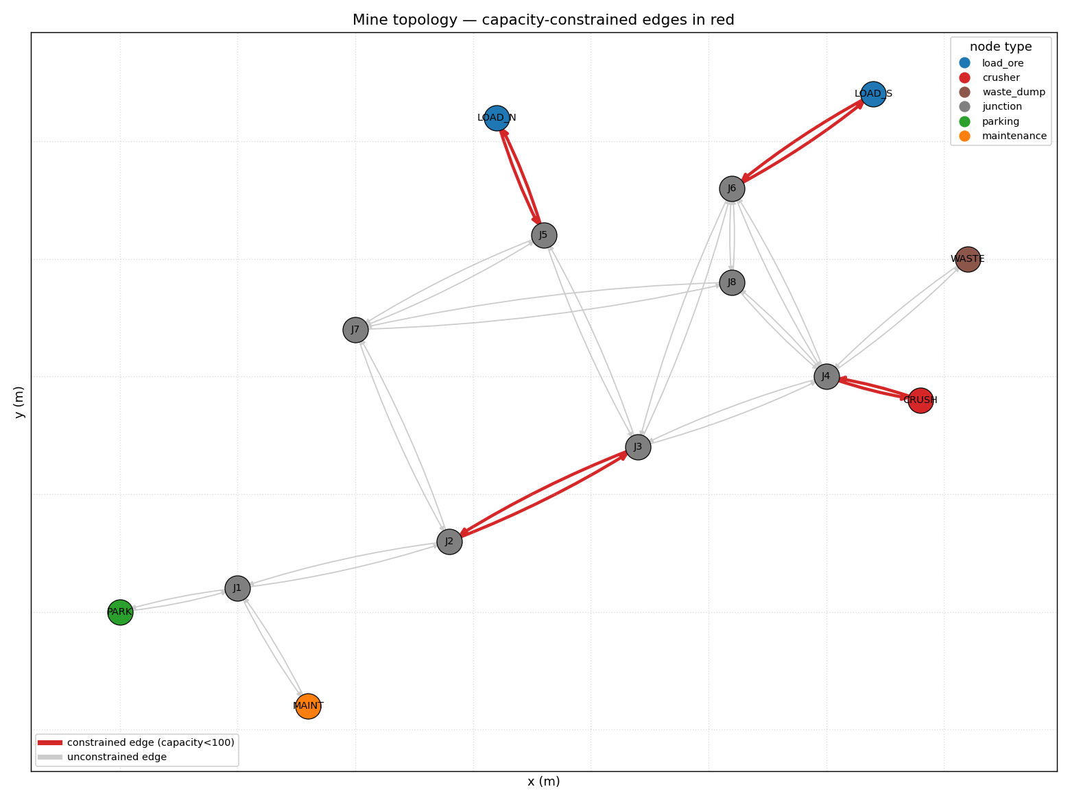
results.csv— per-replication metrics (180 rows for the full sweep).summary.json— per-scenario means, 95 % CIs, top bottlenecks, assumptions and limitations.event_log.csv— every event for every truck in every replication (~430 k rows).topology.png— static diagram of nodes / edges with constrained edges highlighted in red.
3. Reproducibility
Each replication’s RNG is seeded from
SHA-256(base_random_seed :: scenario_id :: replication_index) truncated
to 64 bits. The base seed is read from baseline.yaml
(simulation.base_random_seed = 12345) and inherited by every scenario.
Per-rep seeds appear in results.csv under the random_seed column.
Re-running python run.py produces byte-identical results.csv and
summary.json (timestamp-free outputs) on the same Python / SimPy / NumPy
versions.
4. Conceptual model
See conceptual_model.md for the full conceptual
model. Brief summary:
- Entities: trucks (one SimPy process each).
- Resources: loaders (
L_N,L_S), the crusher dump (D_CRUSH), and seven capacity-constrained edges (E03 ramp ×2, E05 crusher approach ×2, E07 north-pit ×2, E09 south-pit ×2). Edges with capacity ≥ 100 are treated as effectively unlimited and modelled as plainenv.timeout. - Stochasticity: truncated-normal load and dump times, plus a per-edge lognormal travel-time multiplier with unit mean (CV = 0.10).
- Random initial stagger: each truck is dispatched at a uniform
[0, 60] s offset to avoid pathological insertion-order resource
ordering at
t = 0. - End-of-shift policy: no new loader requests after 480 min;
in-flight loaded trucks complete their dump (tonnes counted only at
dump_end).
5. Routing and dispatching
Routing uses networkx.dijkstra_path over the directed graph with
edge weight distance_m / (max_speed_kph × 1000 / 60) (minutes).
Closed edges (closed = true in edges.csv after scenario overrides) are
removed from the graph. Routes are recomputed from the current node at
the start of every empty leg, so closures and per-scenario speed
overrides take effect immediately. If a required route does not exist,
the model raises RoutingError rather than silently producing a misleading
result.
Dispatching follows the baseline nearest_available_loader policy
with shortest_expected_cycle_time tie-breaker:
score(loader) = travel_time(current_node → loader_node)
              + queue_size(loader) × mean_load_time(loader)
The dispatcher picks the loader with the lowest score. Ties are broken by shorter expected return travel from loader to crusher.
This rule is queue-aware — it accounts for the busy time and queue at each loader, not just travel distance — and naturally balances load across both pits.
6. Key results
All values are means over 30 replications; bracketed values are 95 % confidence intervals using Student’s t-distribution (df = 29).
| Scenario | Trucks | Tonnes (mean) | Tonnes / h | Cycle (min) | Crusher util | L_N util | L_S util | Truck util | Loader queue (min) | Crusher queue (min) |
|---|---|---|---|---|---|---|---|---|---|---|
baseline | 8 | 13 143 [13 089 – 13 198] | 1 643 | 30.1 | 0.90 | 0.72 | 0.70 | 0.79 | 2.81 | 3.45 |
trucks_4 | 4 | 7 983 [7 945 – 8 021] | 998 | 24.6 | 0.56 | 0.36 | 0.48 | 0.94 | 0.92 | 0.65 |
trucks_12 | 12 | 13 783 [13 683 – 13 883] | 1 723 | 43.7 | 0.93 | 0.76 | 0.73 | 0.57 | 4.19 | 14.92 |
ramp_upgrade | 8 | 13 173 [13 125 – 13 221] | 1 647 | 30.1 | 0.91 | 0.73 | 0.71 | 0.80 | 2.83 | 3.30 |
crusher_slowdown | 8 | 7 237 [7 154 – 7 320] | 905 | 56.1 | 0.94 | 0.40 | 0.39 | 0.50 | 1.80 | 26.61 |
ramp_closed | 8 | 13 110 [13 043 – 13 177] | 1 639 | 30.2 | 0.90 | 0.72 | 0.71 | 0.79 | 2.80 | 3.41 |
Numbers come straight out of summary.json and can be reproduced with
python run.py.
7. Answers to the operational decision questions
Q1. Expected ore throughput in the baseline 8-hour shift
~13 100 tonnes per shift, or about 1 640 t/h. The 95 % CI is narrow ([13 089 – 13 198]) because the crusher near-saturates and damps stochastic variation in upstream times.
Q2. Likely bottlenecks
- The crusher is the single dominant constraint. Its utilisation sits at 0.90 in the baseline and rises to 0.93–0.94 as soon as the fleet is enlarged or the crusher itself is slowed. Mean crusher queueing time jumps from 3.4 min (baseline) to 14.9 min (12 trucks) to 26.6 min (slow crusher).
- The slow north-pit loader (
L_N, 6.5 min mean load) is a secondary bottleneck. It accumulates a longer mean queue (4.5 min) than the crusher in the baseline because each truck holds it for longer. - The narrow ramp
E03_UP/E03_DOWNis not binding in any of the six scenarios. Empty trucks already prefer the western bypass, and the loaded route via the upper haul road does not require the ramp.
summary.json → scenarios.<id>.top_bottlenecks ranks all resources by
mean queue wait per scenario, drawn from the per-replication queue
statistics.
Q3. Does adding more trucks materially improve throughput?
No — the system saturates near 8 trucks. Adding 4 trucks (4 → 8) adds 5 160 t (+65 %). Adding the next 4 trucks (8 → 12) adds only 640 t (+5 %). Truck utilisation collapses from 0.94 → 0.79 → 0.57 across the 4/8/12 cases, and the crusher’s queue grows from 0.7 to 14.9 min — the extra trucks simply queue at the crusher.
Q4. Would improving the narrow ramp help?
No, not under these scenarios. ramp_upgrade raises ramp speed and
removes the capacity-1 constraint, but throughput is essentially
unchanged (13 173 vs 13 143 t — within the 95 % CI overlap). The crusher
is binding, so freeing the ramp does not unlock more throughput.
The ramp would only matter if (i) the fleet were small enough that travel time dominates, or (ii) the ramp’s capacity-1 constraint actually queued. Neither is the case in the six required scenarios.
Q5. Sensitivity to crusher service time
Very high. Doubling mean dump time from 3.5 → 7.0 min cuts throughput roughly in half (13 143 → 7 237 t, –45 %). This is the largest single- parameter sensitivity in the study and confirms the crusher is the binding resource. Crusher mean queue wait jumps from 3.4 to 26.6 min; loader utilisation falls from ~0.71 to ~0.39 because trucks back up behind the crusher rather than cycling.
Q6. Operational impact of losing the main ramp route
Negligible. With E03_UP and E03_DOWN closed, throughput drops by 0.25 % (13 143 → 13 110 t — within CI overlap). The bypass via J2 → J7 → J5 / J8 is already the shortest empty route from PARK and the loaded route does not depend on the ramp at all (LOAD_N → J5 → J3 → J4 → CRUSH uses upper haul roads, not the ramp). The ramp adds resilience in worse scenarios but, on these data, the bypass is a very close substitute.
8. Behavioural self-checks
The script prints (and the harness re-runs) six broad sanity checks. All six pass on the latest run:
[PASS] trucks_12_gt_trucks_4
[PASS] baseline_gt_trucks_4
[PASS] ramp_upgrade_ge_baseline
[PASS] crusher_slowdown_lt_baseline
[PASS] ramp_closed_le_baseline
[PASS] truck_count_saturation_plausible
9. Limitations
- E03_UP / E03_DOWN as two independent capacity-1 resources slightly understates contention versus a single shared bidirectional channel.
- No truck breakdowns, refuelling, operator breaks, or shift handovers.
- Speed factors are uniform per edge — gradient and curvature are
abstracted into
max_speed_kph. - Travel-time noise is i.i.d. per traversal, so correlated weather or time-of-day effects are not modelled.
- Routes are committed at dispatch time; trucks in flight do not reroute in response to growing queues.
- Loaders and the crusher are 100 % available within the shift.
10. Suggested further scenarios
- Crusher ×2. Add a second dump capacity to the crusher (or a second crusher) to confirm the throughput ceiling moves and to dimension the loaders for the next bottleneck.
- Faster loader at LOAD_N. Shorten the north-pit mean load time to match LOAD_S to test whether evening loader speed reduces queueing.
- Ramp closure + crusher slowdown. Confirm whether the bypass remains adequate when both ramp and crusher are stressed.
- Stochastic loader breakdowns. Introduce reliability with mean time-to-failure and repair, to size the second loader as a hedge.
These are listed for the operator’s consideration and were not implemented in this submission.
11. Repository layout
.
├── conceptual_model.md
├── README.md
├── requirements.txt
├── run.py
├── plot_topology.py
├── src/
│   ├── __init__.py
│   ├── model.py        # data + scenario inheritance + graph + RNG helpers
│   ├── simulation.py   # SimPy resources, truck process, dispatcher, event log
│   ├── experiment.py   # replication driver + scenario sweep
│   └── analysis.py     # CIs, bottleneck identification, output writers
├── data/               # provided inputs (read-only)
│   ├── nodes.csv
│   ├── edges.csv
│   ├── trucks.csv
│   ├── loaders.csv
│   ├── dump_points.csv
│   └── scenarios/
│       ├── baseline.yaml
│       ├── trucks_4.yaml
│       ├── trucks_12.yaml
│       ├── ramp_upgrade.yaml
│       ├── crusher_slowdown.yaml
│       └── ramp_closed.yaml
├── results.csv         # generated
├── summary.json        # generated
├── event_log.csv       # generated
└── topology.png        # generated by plot_topology.py